Deep learning concepts

A neural network are layers of neurons connected by activation functions that transform an input into an output. In between there are different hidden layers which build the logic between input and outputs. The prediction is evaluated via a score function whose result is used to build an optimizer that backpropagates along the network to update neurons weights and minimize the consecutive error.

To avoid biases data is split into train, test and validate blocks. The train test is the one used to compute the networks weights, the validation set is used to compute the unbiased score of the model and to tune hyperparamenters, the test set is used to asses the final score of the model since this data hasen’t been used before.

feed forward

The flow of information is in the forward direction, supervised without feedback.

We take a matrix X on nxm dimensions and a prediction variable y of k elements. We select a weight vector w₁ with l₁ entries and a ReLU function $g_1: ^l ^l $ so that

(g₁(y)) = maxy_i, 0   z₁ = g₁(w₁β+b)

The second and third layers have:

z₂ = g₂(w₂z₁+b₂)   z₃ = g₃(w₃z₂+b₃)

and finally the predicted variable:

$$ \hat y_i = softmax_i(z_3) = \frac{e^{(z_3)_i}}{\sum_j e^{(z_3)_i}} $$

We have therefore to set the parameters: w₁, w₂, w₃, b₁, b₂, b₃

layers

Usually layers used in a network are:

• input: data formatted in tensors
• normalization: predetermined min/max to scale values between [0,1] or [-1,1]
• convolutional: applies NxN filters across NxN neurons around each selected neuron
• pooling: decrease sensitivity to features (usually averaging or taking the max over patches)
• activation: applies activation functions
• dropout: nullify some weights to decrease parameter space
• output: prediction formatted as a tensor

dense - flatten

Flatten From matrix to array

dense(16) + input(5,3) = output(5,16)

input(5,3) + flatten() = input(15) + dense(16) = output(16)

batch

The total number of examples in a training iteration

activation functions

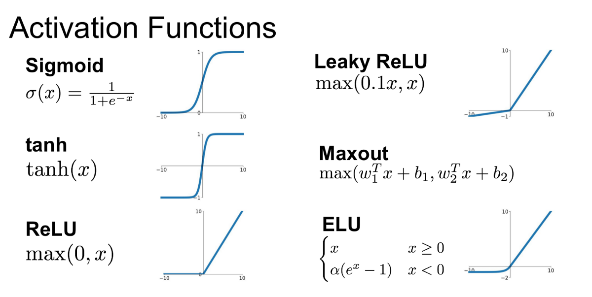
Activation functions are used to connect neurons between networks. Usually the activation functions is constant througout the hidden layer and might vary at the output layer. The main reason to select an activation function for the output layer is the domain of the output variable:

• binary classification: sigmoid
• multiclass: softmax
• multilabel: sigmoid

A key feature for the activation function is derivability since backpropagation requires at least the first derivate of the function.

list of activation functions

Sigmoid / Logistic Advantages

Smooth gradient, preventing “jumps” in output values. Output values bound between 0 and 1, normalizing the output of each neuron. Clear predictions—For X above 2 or below -2, tends to bring the Y value (the prediction) to the edge of the curve, very close to 1 or 0. This enables clear predictions.

Disadvantages

Vanishing gradient—for very high or very low values of X, there is almost no change to the prediction, causing a vanishing gradient problem. This can result in the network refusing to learn further, or being too slow to reach an accurate prediction. Outputs not zero centered. Computationally expensive

TanH / Hyperbolic Tangent Advantages

Zero centered—making it easier to model inputs that have strongly negative, neutral, and strongly positive values. Otherwise like the Sigmoid function.

Disadvantages

Like the Sigmoid function

ReLU (Rectified Linear Unit) Advantages

Computationally efficient—allows the network to converge very quickly Non-linear—although it looks like a linear function, ReLU has a derivative function and allows for backpropagation

Disadvantages

The Dying ReLU problem—when inputs approach zero, or are negative, the gradient of the function becomes zero, the network cannot perform backpropagation and cannot learn.

Leaky ReLU Advantages

Prevents dying ReLU problem—this variation of ReLU has a small positive slope in the negative area, so it does enable backpropagation, even for negative input values Otherwise like ReLU

Disadvantages

Results not consistent—leaky ReLU does not provide consistent predictions for negative input values.

Parametric ReLU Advantages

Allows the negative slope to be learned—unlike leaky ReLU, this function provides the slope of the negative part of the function as an argument. It is, therefore, possible to perform backpropagation and learn the most appropriate value of α. Otherwise like ReLU

Disadvantages

May perform differently for different problems.

Softmax e^x/sum(e^x) which resemples Boltzmann probability Advantages

Able to handle multiple classes only one class in other activation functions—normalizes the outputs for each class between 0 and 1, and divides by their sum, giving the probability of the input value being in a specific class. Useful for output neurons—typically Softmax is used only for the output layer, for neural networks that need to classify inputs into multiple categories.

Swish

Swish is a new, self-gated activation function discovered by researchers at Google. According to their paper, it performs better than ReLU with a similar level of computational efficiency. In experiments on ImageNet with identical models running ReLU and Swish, the new function achieved top -1 classification accuracy 0.6-0.9% higher.

cost function

A function that evaluates the error between the fit function and the variable to predict

Squared error (regressions)

F(x,y) = ∑_i(y_i−w_ix)²/N

Logistic function

F(x,y) = ∑_ilog(1+e^{−y_i(w_iTx+b_i)})

cross entropy loss (regressions)

Gini impurity

Hinge loss (support vector machine)

Exponential loss (ada boost)

scores

To evaluate the quality of a model different scores are use to evaluate the predicitons

• Classification Accuracy: percentage of corrected predictions (diagonal elements in the confusion matrix)
• sensitivity: TP/(FN+TP), specificity: TN/(TN+FP)
• precision: TP/(TP+FP), recall: TP/(TP+FN)
• F1 Score: 2/(1/precision+1/recall)
• Logarithmic Loss: $$\frac{1}{N}\sum_i\sum_j y_{ij} \log(p_{ij}) $$
• Area under Curve: The integral of the area between TP and FP
• Mean Absolute Error: $$\frac{1}{N}\sum_i |\hat{y} - y_i| $$
• Mean Squared Error: $$\frac{1}{N}\sum_i (\hat{y} - y_i)^2 $$
• language models: rouge score

backpropagation

Backpropagation is when after running a prediction the error/cost is evaluated. The cost function is derived using an optimizer which runs trhough the neurons of the network changing the neurons weights to minimize the next iteration error.

optimizer

The optimizer suggests the direction for the minimization of the cost function

min_xF(x) := ∑_if_i(x)

Minimize the cost function f(x,y), first order optimizers use the gradient, the second the Hessian.

• gradient

  • first derivative of the cost function
  • move the parameters a step towards the steepest descent with a momentum η $$ \eta \gradient F(x) $$

• Hessian $$ H^2 := \sum_{j} \gradient f_{ij} (x_j) \gradient f_{ij} (x_j)^T $$

• Preconditioner B := diagH

• gradient descent

  • gradient on a random point $$ x_{t+1} = x_t - \eta \gradient F(x_i) $$

• stochastic gradient descent

  • gradient on a random batch $$ x_{t+1} = x_t - \eta_t \gradient f(x_i) $$

• adagrad

  • better performances after some step threshold, more stable
  • independent on η $$ x_{x+1} = x_t - \eta B_t^{-1} \gradient f_i (x_t) $$

bias/variance

Models can have good scores but the solver might be still too inaccurate for the complexity of the problem (over-simplifying over-complicating). The two cases are:

• bias (underfitting): we introduce a pnality bias in the loss to get less significance on the feature
• variance (overfitting): a pure variance optimization leads to complex solutions

The usual practice is to adapt the number of parameters to the complexity of the problem but there are other regularisation techniques to use.

We can use the weight decay where the square of the weights are considered in the loss function.

We can use dropouts which deactives a portion of the neurons to let the optimizer practically modify the architecture.

feature regularisation

Regularisation adds penality to model complexity to decrease overfitting problems.

The main types of regularizations are:

• L1: lasso regularisation (absolute value)
• L2: ridge regularisation (mean squared value)
• Elastic net: combines L1 and L2
• prune: remove branches of trees

L1: ∑_i(y_i−∑_jx_ijβ_j)² + λ∑_j|β_j|

L2: ∑_i(y_i−∑_jx_ijβ_j)² + λ∑_jβ_j²

L1 is shrinks the least important features to zero and it’s suited for feature selection. λ is an hyperparameter to tune. L1 gradient is independent of parameters and therefore their weight can vanish.

Ridge regression is useful when there are few data points compared to features and helps in reducing feature significance.

dropout

Cuts connections when the weight is low, helps against overfitting.

Binary classification

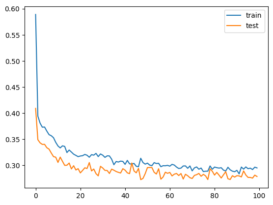
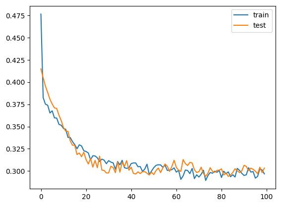
Not performant, dropout 20:

Just about right, dropout 30:

Overfitting, dropout 50:

data augmentation

Some models and algorithms are useful to increase the dataset for extended training purposes data augmentation.

A classical example concerning computer vision is to iterate all available images and make copies after rotation, subset, filtering of those to increase the cases of non-standard takes.

batch normalization

During training batches can be normalized in case a sampling of the dataset can create big distortions in the distribution of min/max values. More on batch normalization

GAN

A separated article on GANs showing how the adversarial architecture helps creating realistic fakes and some keras implementations.

transformers

Transformes use an encode-decode architecture to reduce the input parameter space. The most significant change compared to previous architectures are the attention layers and the enhanced emmbeddings.