
Why quality?

Quotation from Deming
Knowledge of variation: the range and causes of variation in quality, and use of statistical sampling in measurements; Improve constantly and forever the system of production and service, to improve quality and productivity, and thus constantly decrease costs. Break down barriers between departments. People in research, design, sales, and production must work as a team, to foresee problems of production and usage that may be encountered with the product or service. In god we trust, everybody else bring data
We take one location 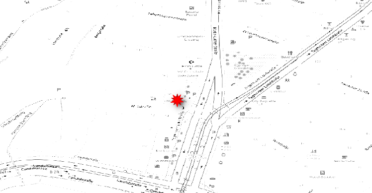 example of a
location
We download the local street network 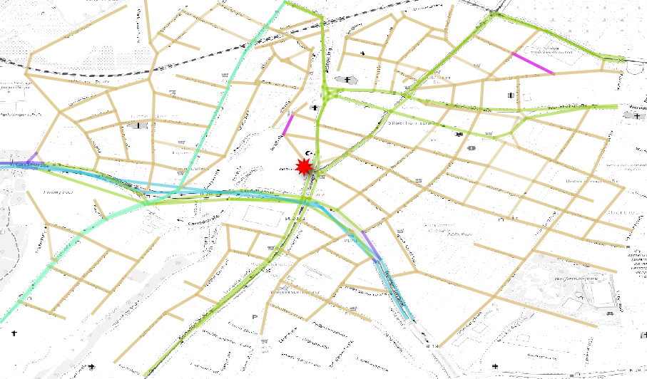 local network
We download the cell coverage in the network area 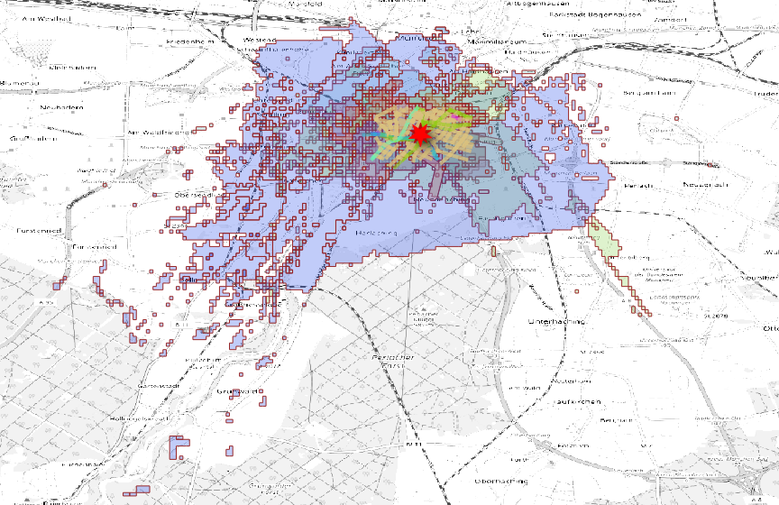 cell coverage around the location
We classify the cells by radius and we plot the coverage centroid
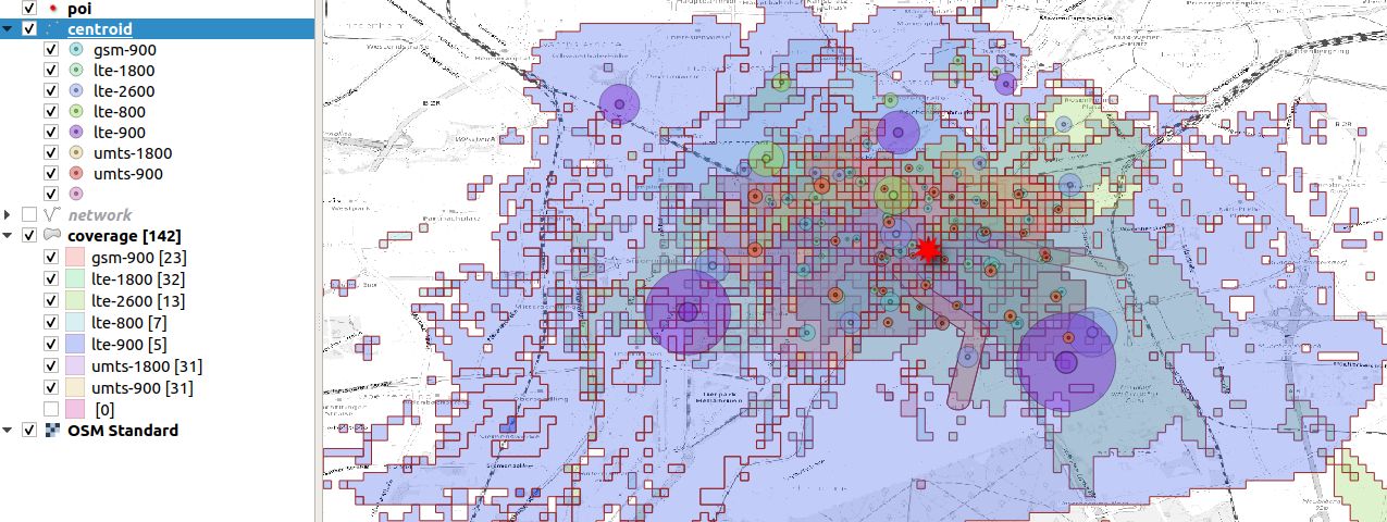 display cells by technology wich influences
the area
We select the most precise cells, some of them happen to be subway
cells 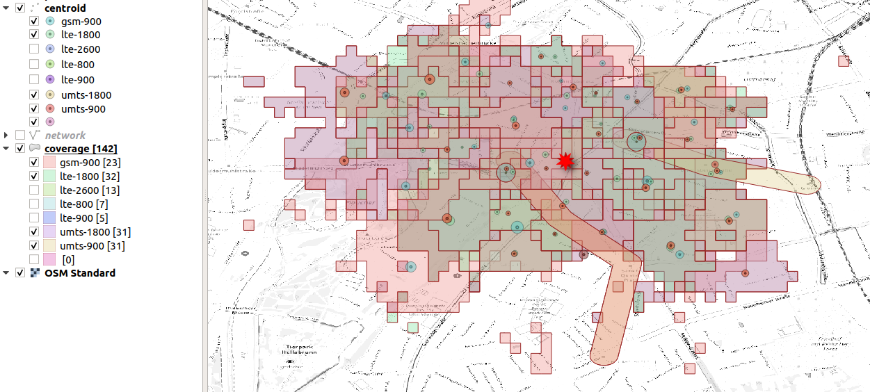 selection of the techologies with good spatial
resolution
We can simplify the geometries taking only the closest and most
precise cells centroids 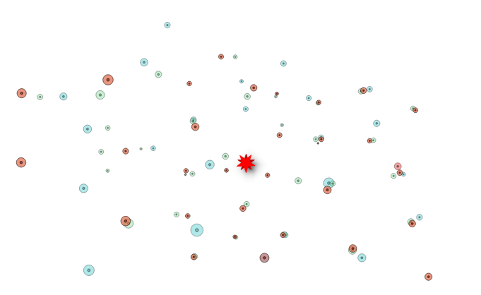 neighboring
cells represented by centroid and radius
and than we try to sum up a portion of activities into some geometries
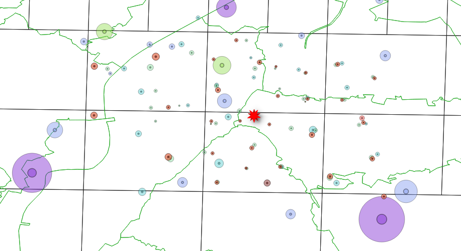 we map the location into a geometry (mtc,
zip5)
But for some technology we have centroids outside the coverage area
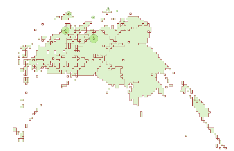 some centroids
are not contained in any area
We want to evaluate count stability using the dominant cell method.
The first test is done moving the center of the overlapping mapping by a displacement (in meters)
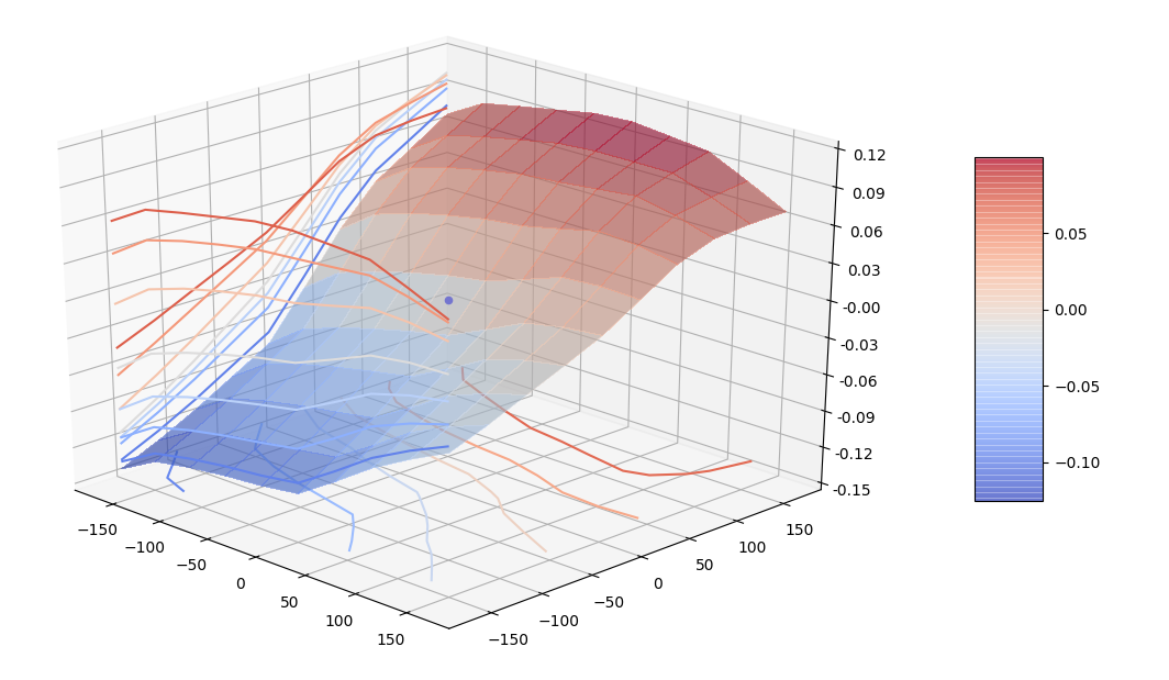 stability of counts after displacement
We than check the stability of counts by area
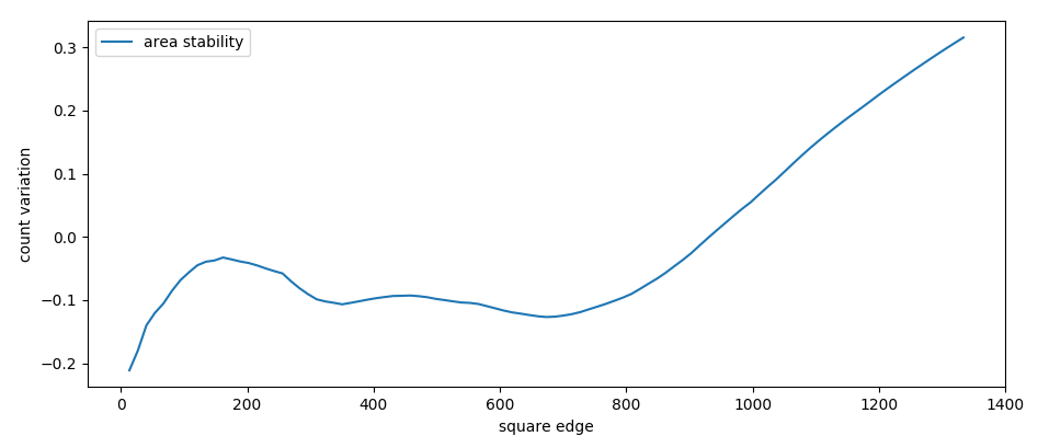 stability of counts after area increase
(edge in meters)
Number of counts strongly increase with mapping area (until 50%).
An activity is made of many events. Currently we
define the dominant cell as the cell where most of the events
took place. For every cell we assign a position which is the centroid of
the BSE (Best Server Estimation), an estimation of the area
where the cell has the best ground coverage without intersection of
other cells with the same technology. Hence, each activity position is
located at the centroid of each dominant cell. 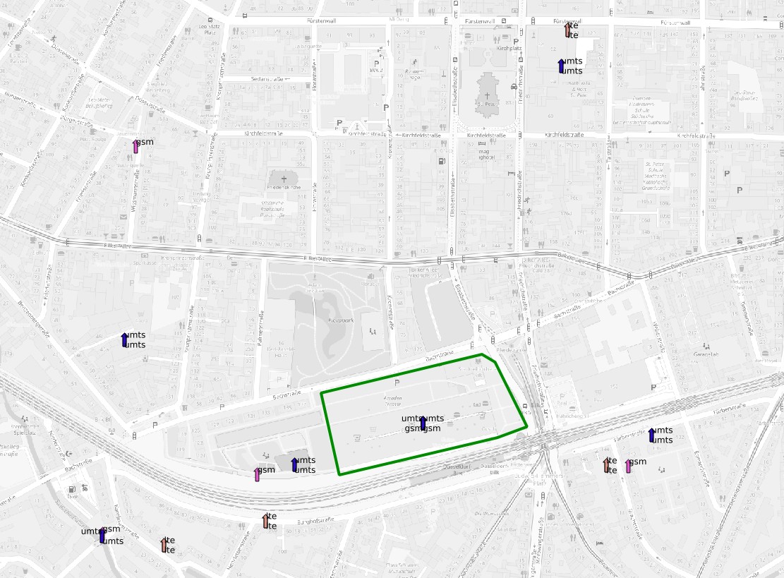 The polygon shows the location we want to
isolate, the arrows the neighbouring cell centroids
The density profile of the activities is then centered around the
centroid position. 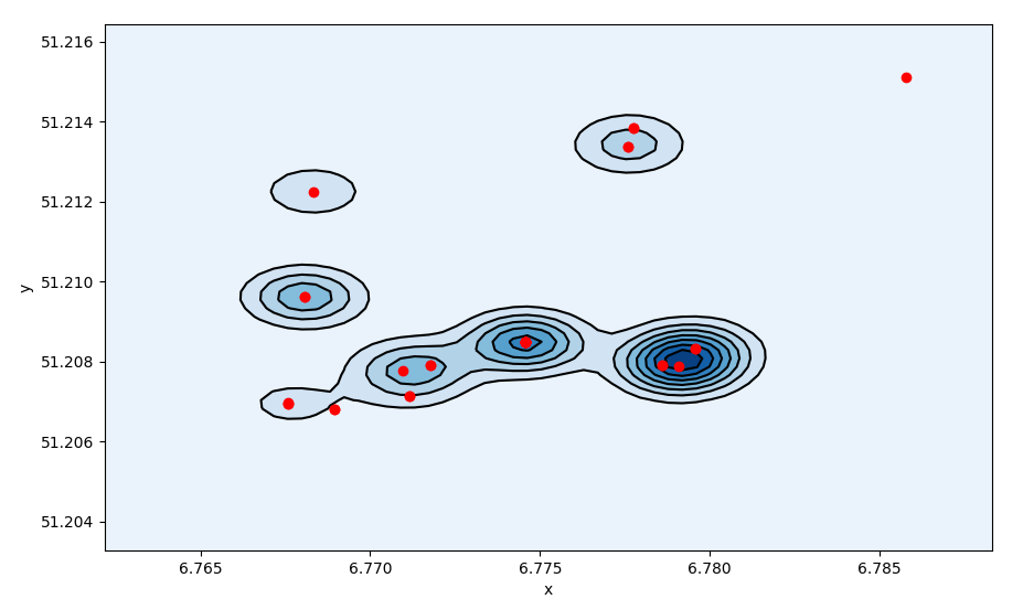
We can divide the space where each cell centroid sits at the vertex
of a Delaunay triangle. 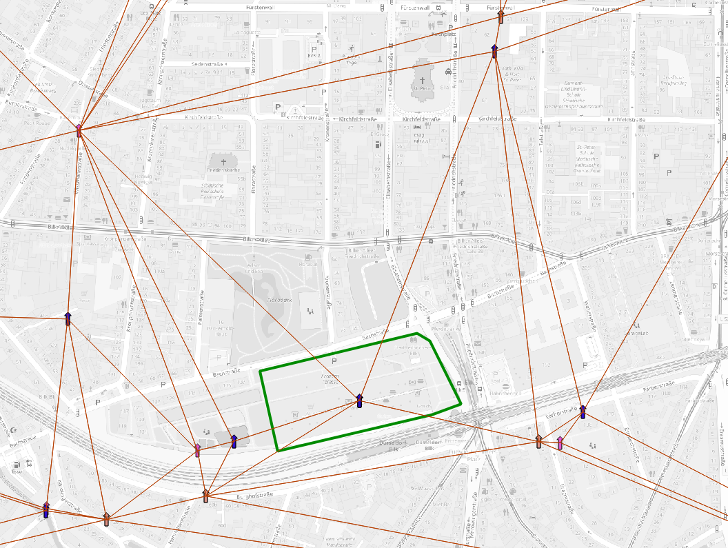 Delaunay
triangulation on cell centroids
If we average over all vertex positions we have a more sparse activity distribution. We can even define a standard error for each activity filter_activities.py. $$ s_x = \sqrt{\frac{ \sum_i (\hat x - x_i)^2 }{N-2}} \qquad s_r = \sqrt{s_x^2 + s_y^2} $$ The standard error define the uncertanty on the activity position.
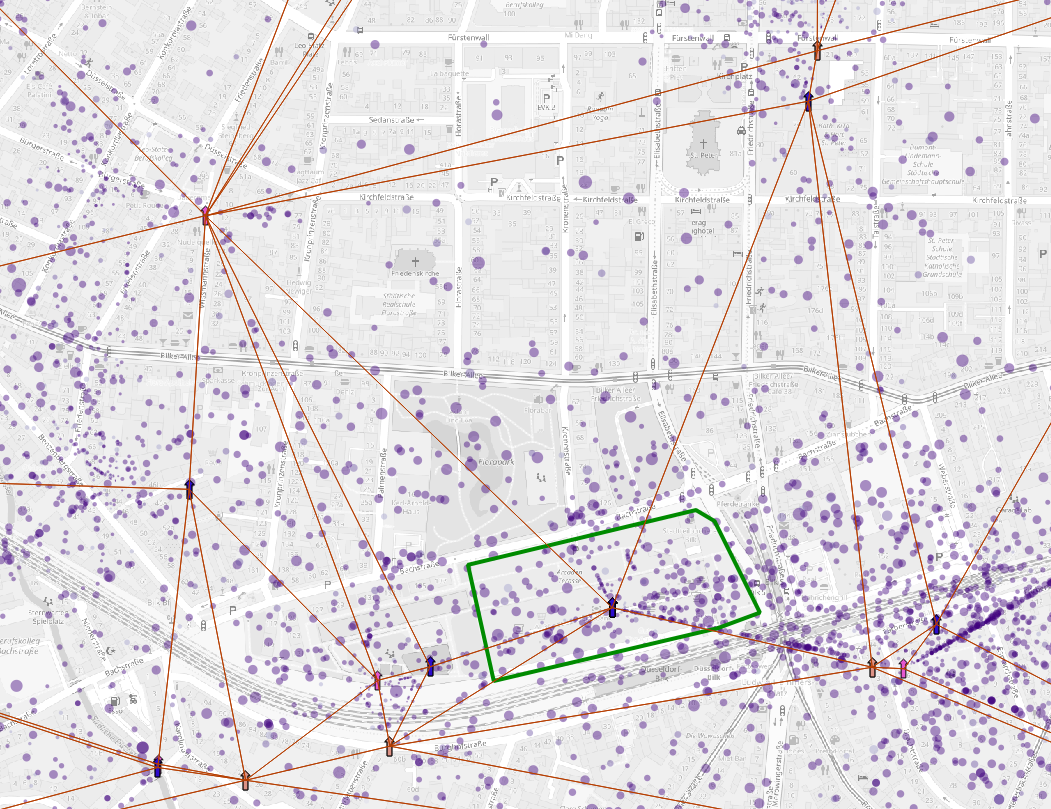 The dots
represent the average activity position, the dot size represent the
standard error of the position
Which translate in a broader density profile. 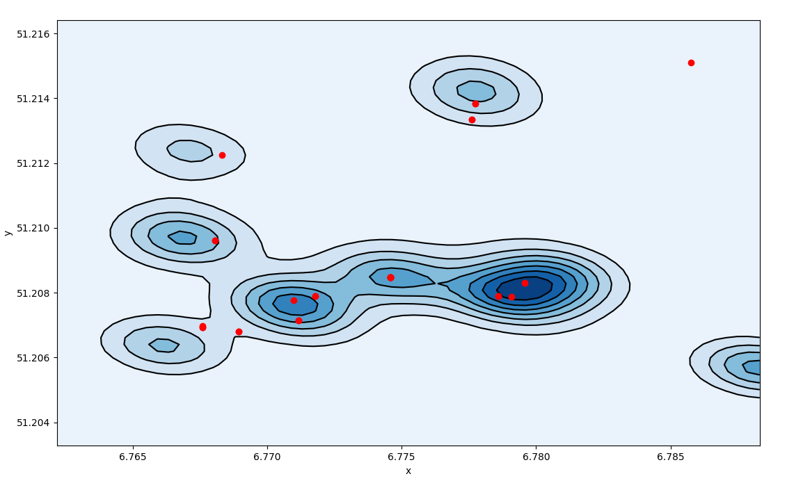 Density profile of triangulated activities,
density spreads over the space
For each polygon we take the distribution of standard error of the
positions inside the polygon. 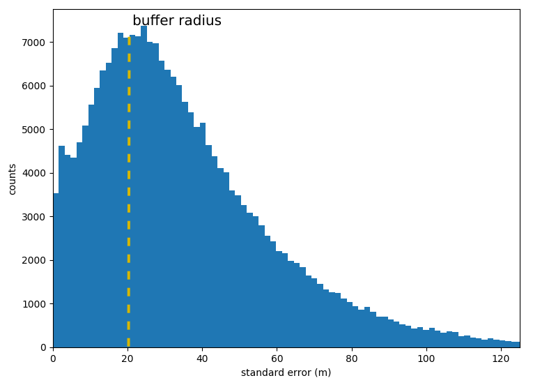 distribution of the
standard errors all over the activities
The median of the standard error distribution defines a buffer radius
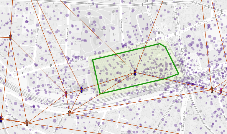 The buffer radius (in green) circulates around
the polygon defining the precision of activity positions per
location
To overcome anonymization problems we transform coordinates in geohash.
Geohash is a indexed short string which contains information about the position and the bounding box of a square. The number of digits sets the precision (i.e. the size of the bounding box) using a octree. Neighbouring boxes have similar indices.
2d representation of an octree
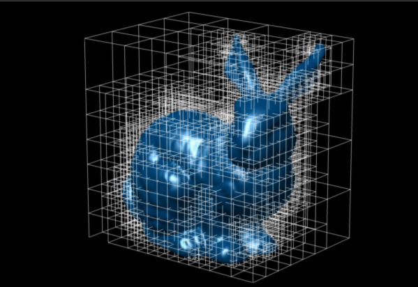 3d usage of an octree
To anonymize the data we loop until we find the minimum number of digits for each geohash string: fenics_finite.py.
vact.loc[:,"geohash"] = vact[['x_n','y_n']].apply(lambda x: geohash.encode(x[0],x[1],precision=8),axis=1)
def clampF(x):
    return pd.Series({"n":sum(x['n']),"sr":np.mean(x['sr'])})
lact = vact.groupby('geohash').apply(clampF).reset_index()
for i in range(3):
    setL = lact['n'] < 30.
    lact.loc[:,"geohash2"] = lact['geohash']
    lact.loc[setL,"geohash"] = lact.loc[setL,'geohash2'].apply(lambda x: x[:(8-i-1)])
    lact = lact.groupby('geohash').apply(clampF).reset_index()
At the end we produce a table similar to this one:
| geohash | count | deviation |
|---|---|---|
| t1hqt | 34 | 0.1 |
| t1hqt3 | 42 | 0.4 |
| t1hqt3zm | 84 | 0.8 |
| t1hqt6 | 44 | 0.6 |
| t1hqt8 | 78 | 0.8 |
| t1hqt9 | 125 | 0.6 |
| t1hqt96 | 73 | 0.3 |
| t1hqt97 | 38 | 0.5 |
| t1hqt99 | 46 | 0.4 |
In post processing we can then reconstruct the geometry: 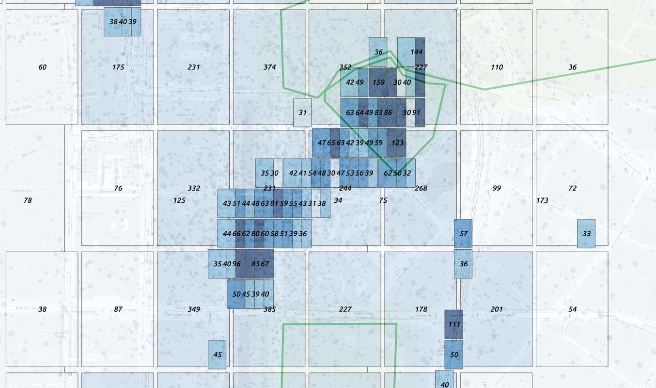 Overcome the anonimization problem using
geohash binning
This allows us to have the larger precision allowded without count loss.
For each box we can estimate the precision 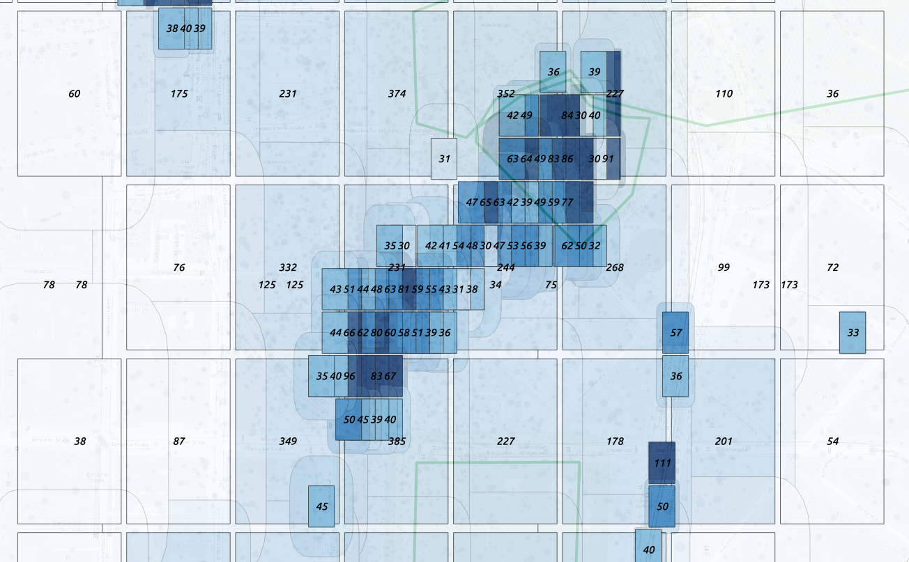 Overcome the anonimization problem using
geohash binning
Alternatively we can apply a double binary octree 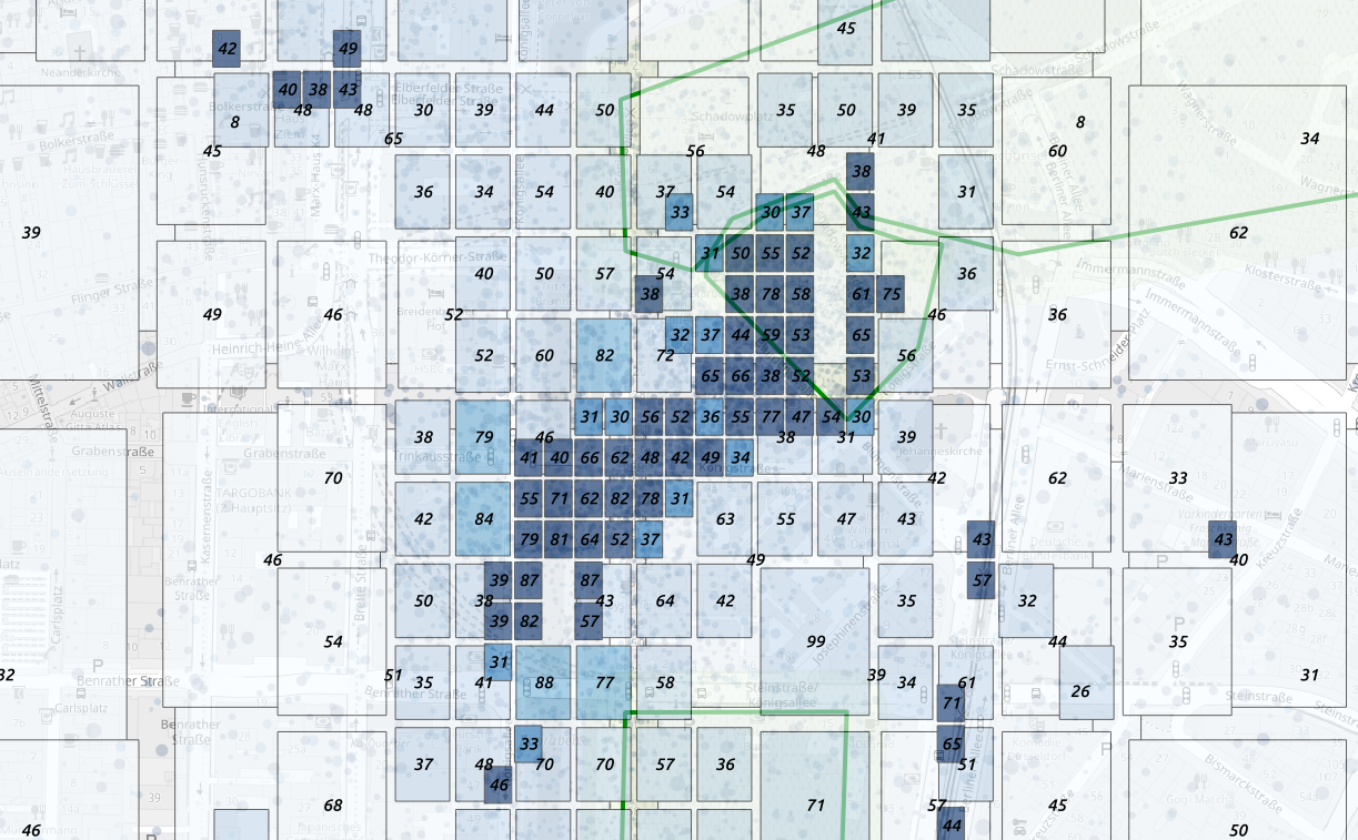 counts on a octree binning
Advantages * no mapping * no BSE * no data loss * custom geometries (postprocessing - no deploy) * no double counting * highest allowed resolution
Cons * no unique counts per polygon * postprocessing always required * land use mapping might have more accuracy
evolution of
mappings
Which was calculated by a simple halfing of each edge:
   BBox = [5.866,47.2704,15.0377,55.0574]
    spaceId = ''
    for i in range(precision):
        marginW = marginH = 0b00
        dH = (BBox[3] - BBox[1])*.5
        dW = (BBox[2] - BBox[0])*.5
        if x < (BBox[0] + dW):
            BBox[2] = BBox[2] - dW
        else:
            marginW = 0b01
            BBox[0] = BBox[0] + dW
        if y < (BBox[1] + dH):
            BBox[3] = BBox[3] - dH
        else:
            marginH = 0b10
            BBox[1] = BBox[1] + dH
        spaceId = spaceId + str(marginW + marginH)
In post processing we can reconstruct the geometry and interpolate the missing boxes.
The spatial resolution is given by the distribution of cells which modifies the definition of space around. We represent each cell centroid as a trapezoid whose center corresponds to the cell centroid and the area to a portion of the BSE area fenics_finite.py. We define an Helfrich Hamiltonian on a manifold: z = z(x,y) to define the curvature of space caused by the cell position: $$ F(z) = \frac{1}{2} \int d x d y (k_{ben}(\nabla^2 z)^2 + k_{stif} (\nabla z)^2 ) $$ Where the bending and stiffness parameters are controlled by the parameters kben and kstif.
To solve the equation we chose a square mesh and we apply finite differences method on the lattice representing the space. The solution of the equation is done numerically applying a Jacobi iteration on a 5x5 square matrix to convolve with the square lattice representing the space. kben and kstif represent the weights for the Laplacian Δ and the square Laplacian term Δ2.
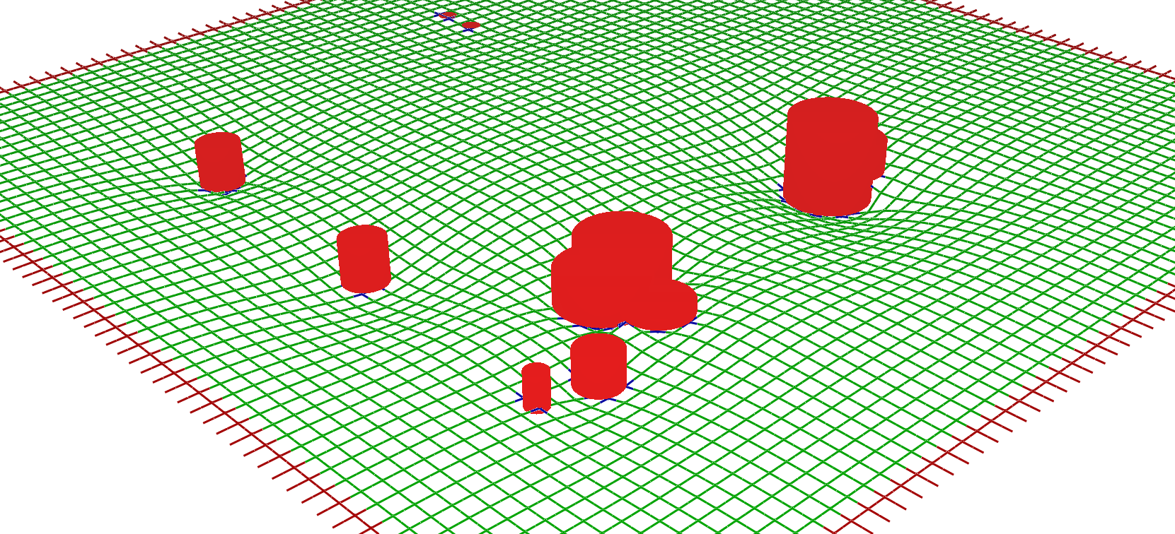 Solution of the Helfrich Hamiltonian on a square
lattice, the cylinders represent the cell centroids The boundary
conditions and the constraints are given by the red and blue beads which
are not moved during the iterations. We can increase the resolution
interpolating the lattice points.
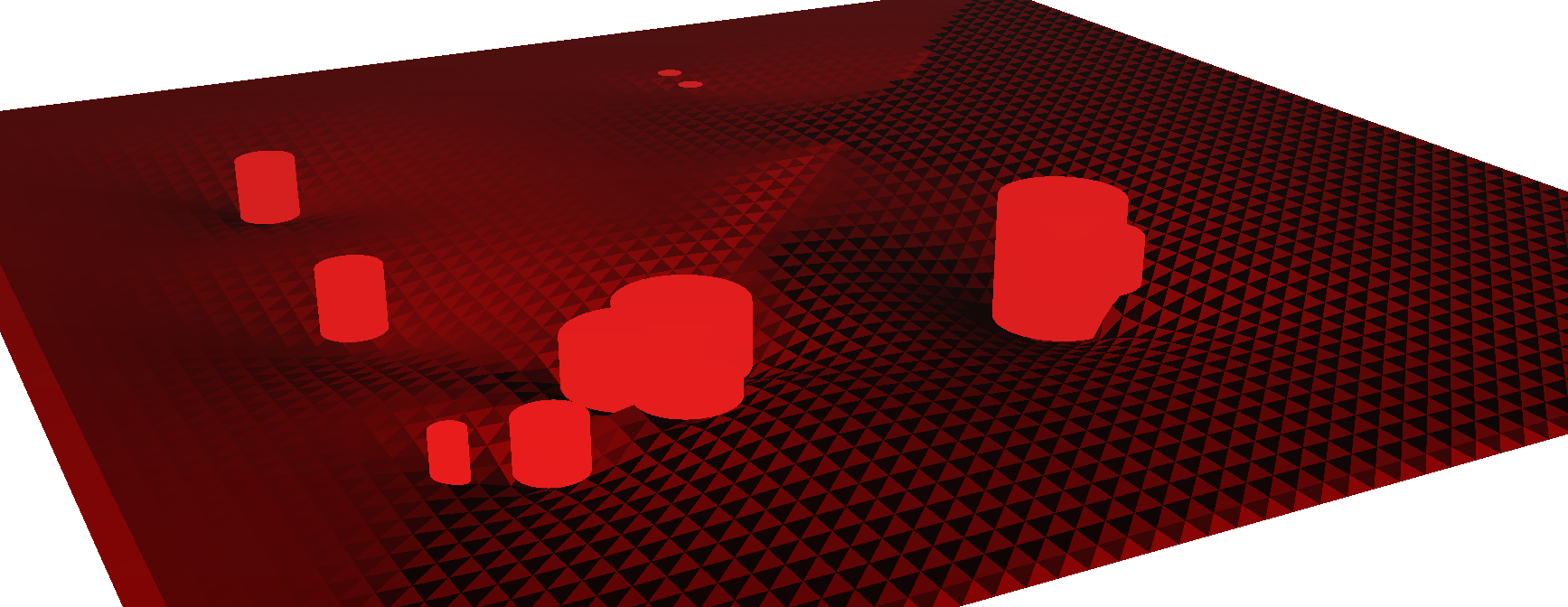 discretization of the lattice solution
To normalize the effect of the space curvature on the activity positions we move each activity by the gradient of the space deformation $$ \nabla z = \frac{\partial z}{\partial x} \hat x+ \frac{\partial z}{\partial y} \hat y $$
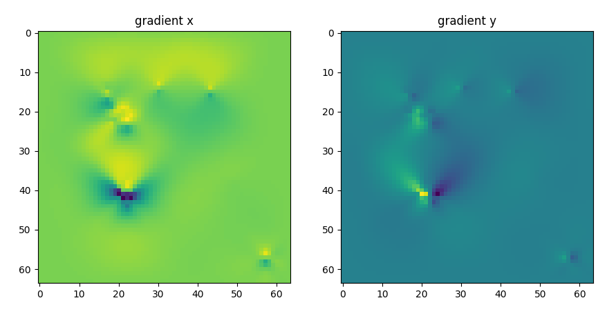 gradient of the space deformation on the x and y directions
If we invert the gradiant we obtain the displacement induced by the
cell geography 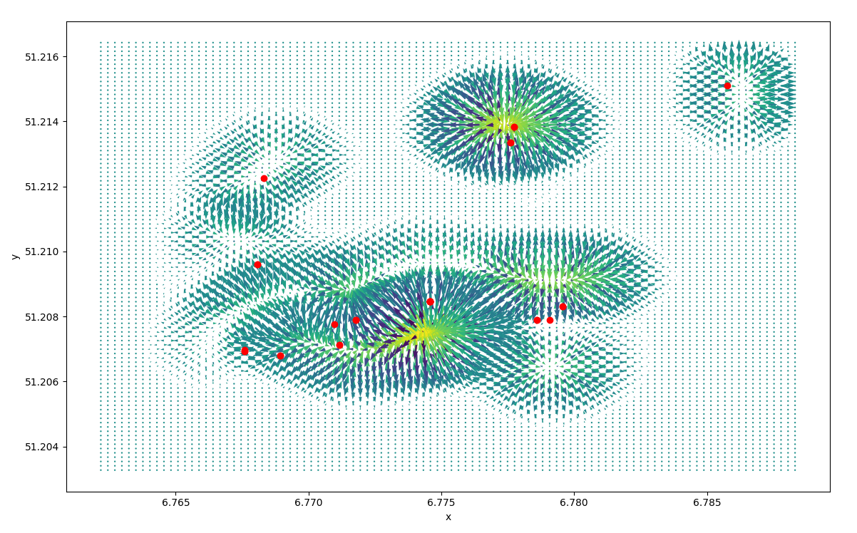 vector field of
the displacement and centroids
We can see how the single activities have moved. 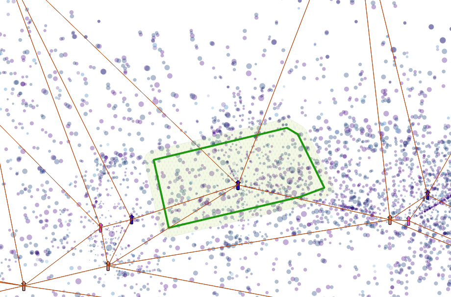 shift of activities, purple to blue
We then recalculate the density plot based on the new positions.
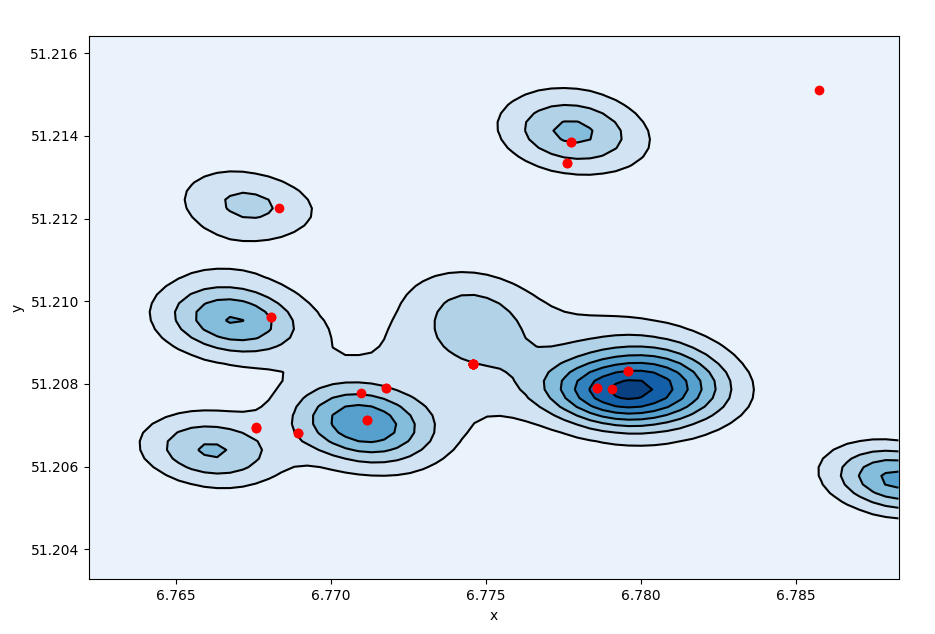 density plot after displacement
We move the single activities according to the gradient. 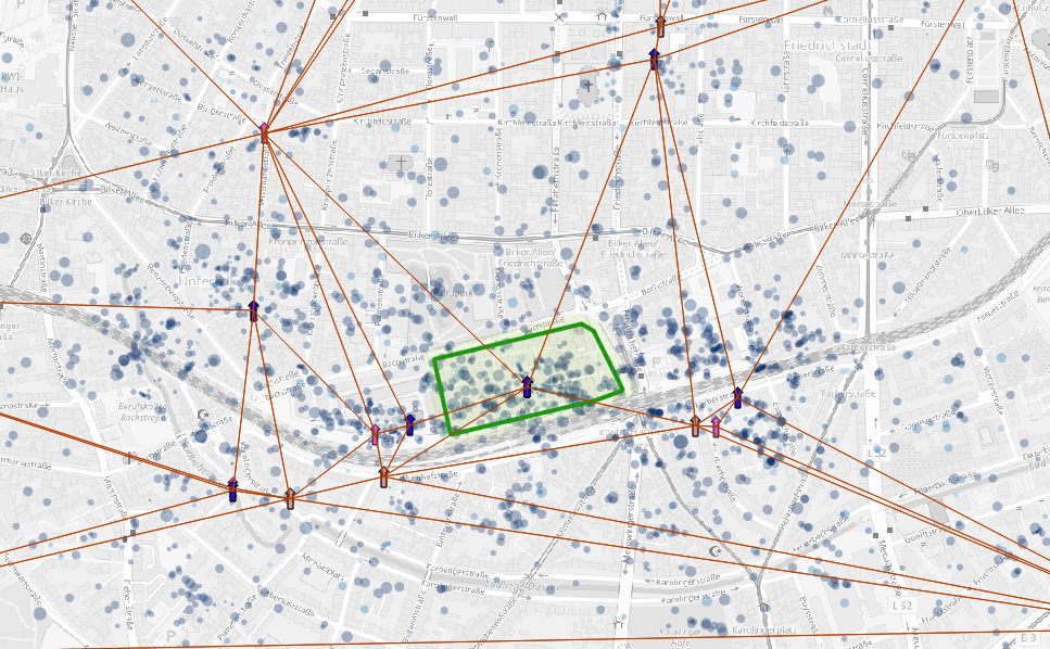 new activity position after
displacement
On top of the cell space distortion we apply the underlying network
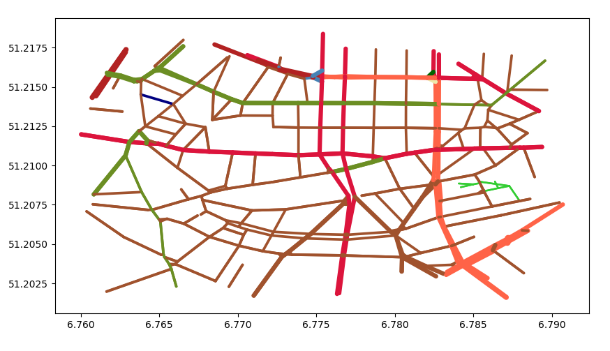 underlying netwok, each street class has a
different color
We discretize the network, apply a width depending on the street
speed and apply a smooting filter. 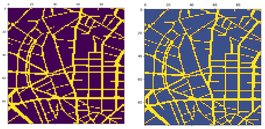 smoothed filter on network
Similarly we can create a displacement map based on the street
network. 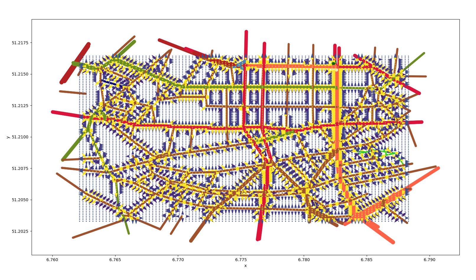 displacement due to
the street network
To summarise the whole scheme of the procedure is described in this
scheme: 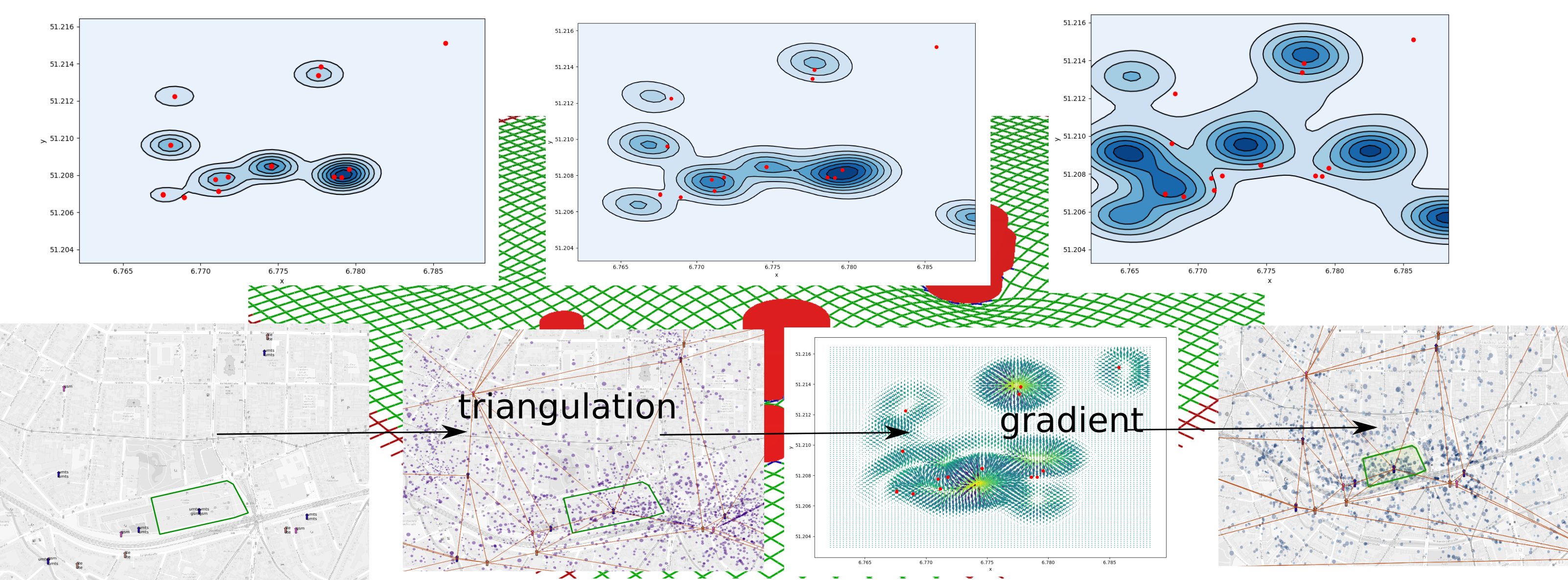 density plot after each operation and overview on the
procedure
The procedure show how to create a more realistic density plots. Further tuning is necessary.
Finally we update the mapping etl_roda.py.
