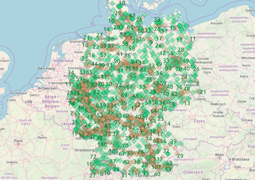
 BaSt Germany for motorways and primary
streets
BaSt Germany for motorways and primary
streetsAcross germany there are thousands of counting locations on the main roads and the count of vehicle crossing the section of the street is public
 BaSt Germany for motorways and primary
streets
For each of those location we select a pair of openstreetmap nodes (arrows) for the same street class.
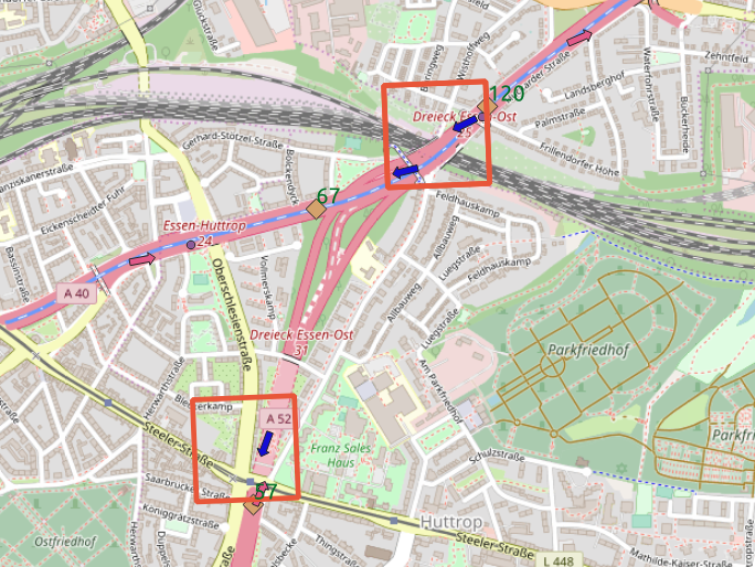 For the same
BaSt location the tile intersects more streets
To stabilize over year we build an isocalendar which represents each date as week number and weekday. We see that isocalendar is pretty much stable over the year with exception of easter time (which shifts a lot).
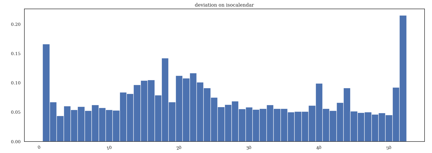 standard
deviation on same isocalendar day over the year
We take hourly values of BaSt counts and we split in weeks. Every week is represented as an image of 7x24 pixels.
 image representation of time series
The idea is to profit from the performances of convolutional neural networks to train an autoencoder and learn from the periodicity of each counting location.
Convolutional neural network usually work with larger image sizes and they suffer from boundary conditions that creates a lot of artifacts.
That’s why we introduce backfold as the operation of adding a strip to the border from the opposite edge.
 backfolding the image
In this way we obtain a new set of images (9x26 pixels)
 image representation of time series with
backfold
And produce a set of images for the autoencoder
 image dataset
We first define a short convolutional neural network
 short convNet in 3d
We than define a slightly more complex network
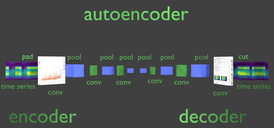 definition of a conv net in 3d
In case of 7x24 pixel matrices we adjust the padding to achieve the same dimensions.
We fit the model and check the training history.
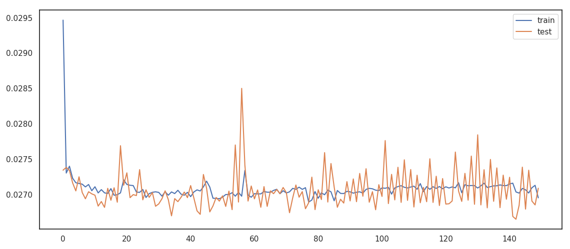 training history
Around 300 epochs the model is pretty stavle and we can see the morphing of the original pictures into the predicted
 raw image morphed into decoded one, no
backfold
If we introduce backfold we have a slightly more accurate predictions
 raw image morphed
into decoded one, with backfold
The most complex solution comes with the deeper model
 morphing for convNet
At first we look at the results of the non backfolded time series
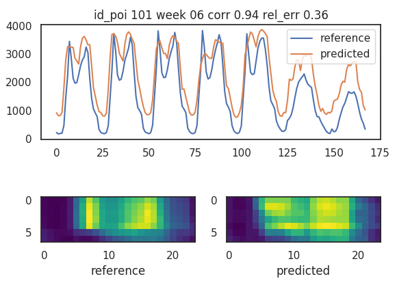 results for the short
convolution, no backfold
If we add backfold we improve correlation and relative error
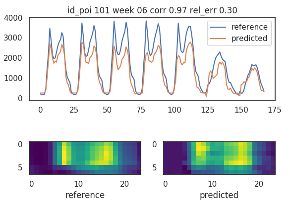 results for the short convolution
The deepest network improves significantly the relative error but as a trade off loose in correlation
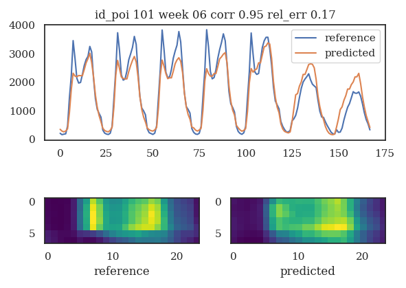 convNet results with backfold
The deepest network improves drastically the relative error sacrifying the correlation
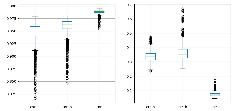 boxplot correlation and error difference
between models
Correlation not being in the loss function is really disperse while optimizing
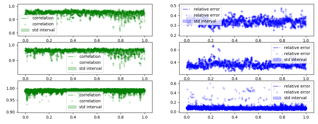 confidence
interval for correlation and relative error
Ranking is not stable among the different methods
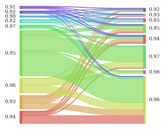 Sankey diagram of correlation shift between
different methods
Different methods behave differently wrt the particular location
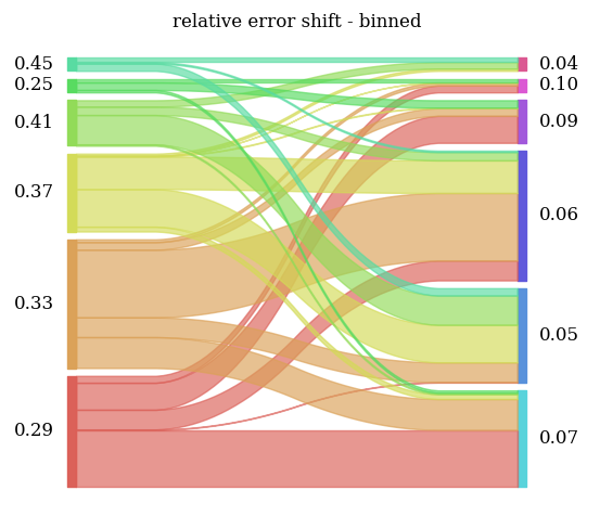 sankey diagram of error reshuffling
The deepest network tend to amplify the bad performances in correlation
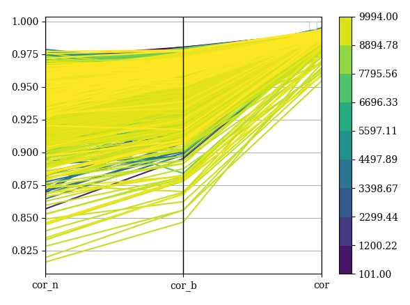 parallel diagram of
correlation differences
The short backfolded model has the worse performances for locations that had the best performances in the non backfolded version
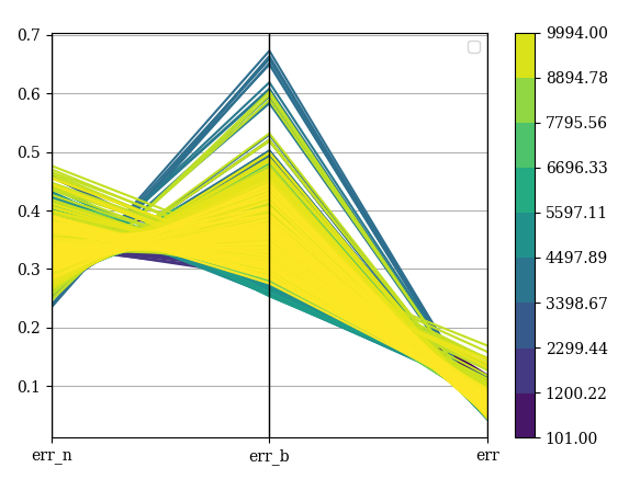 parallel diagram of relative error
We perform a dictionary learning for knowing the minimal set average of time series to describe with good accuracy any location. For that we will use a KMeans
clusterer = KMeans(copy_x=True,init='k-means++',max_iter=600,n_clusters=4,n_init=10,n_jobs=1,precompute_distances='auto',random_state=None,tol=0.0001,verbose=2)
yL = np.reshape(YL,(len(YL),YL.shape[1]*YL.shape[2]))
mod = clusterer.fit(yL)
centroids = clusterer.cluster_centers_
We start with the most common time series and we calulate the score of all locations on that cluster
 most frequent cluster
We realize the 90% of the locations and weeks have a correlation higher than 0.9
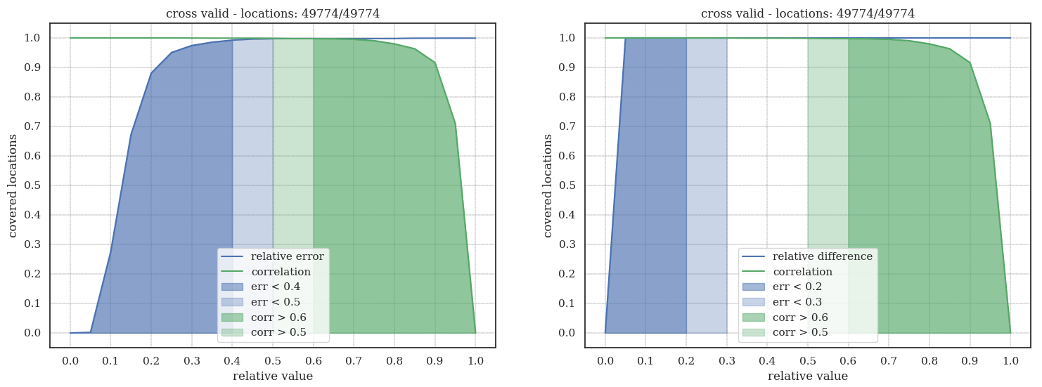 kpi
distribution for single cluster
A single cluster is already a good description for any other location but we want to gain more insight about the system. We than move the 2 clusters to classify the most important distintion between locations which we will call “touristic” and “commuter” street classes.
 most 2 frequent clusters, touristic and
commuter
We can extend the number of cluster but we don’t significantly improve performances but land to same extreme cases
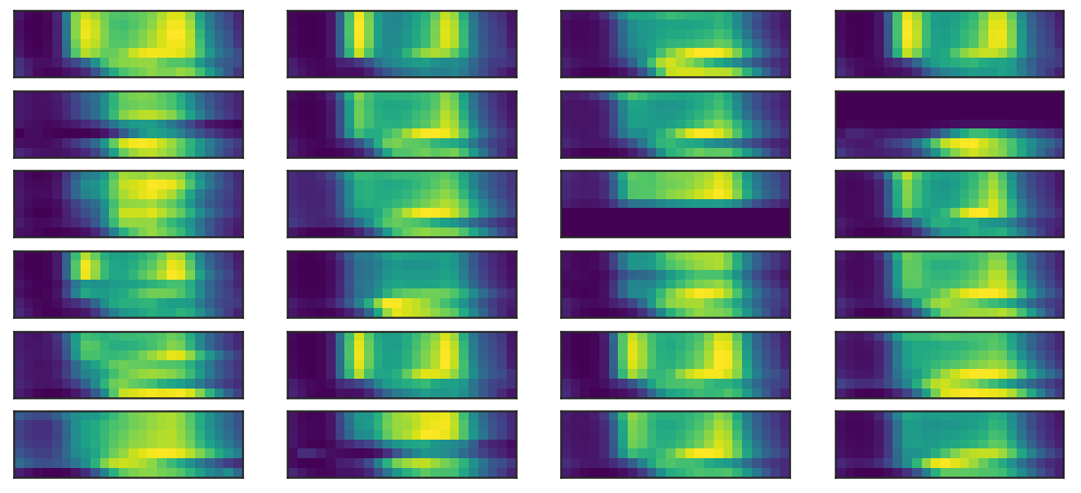 most 24 frequent clusters
If we look at the KPIs distribution 4 clusters are the best trade-off between precision and computation
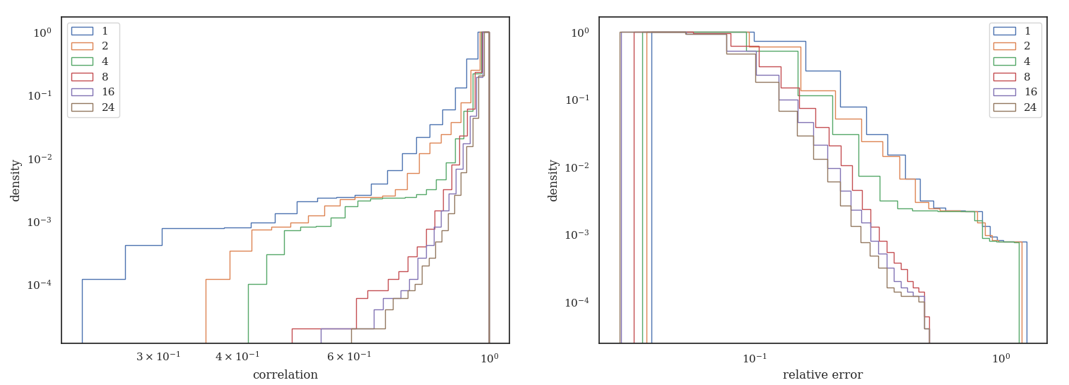 histogram for
correlation and relative error
If we look at the most 4 frequent clusters we see that they are split in 2 touristic and 2 commuters
 most 4 frequent clusters
We want than to see how often a single location can swap between commuter and touristic and we see that locations are strongly polarized though all the year
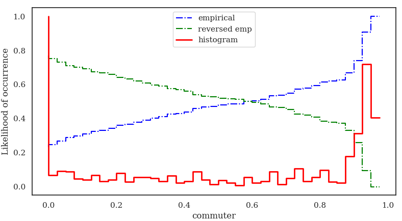 cluster
polarization
If we look at the weekly distribution we see that the commuting pattern ressamble our expectation
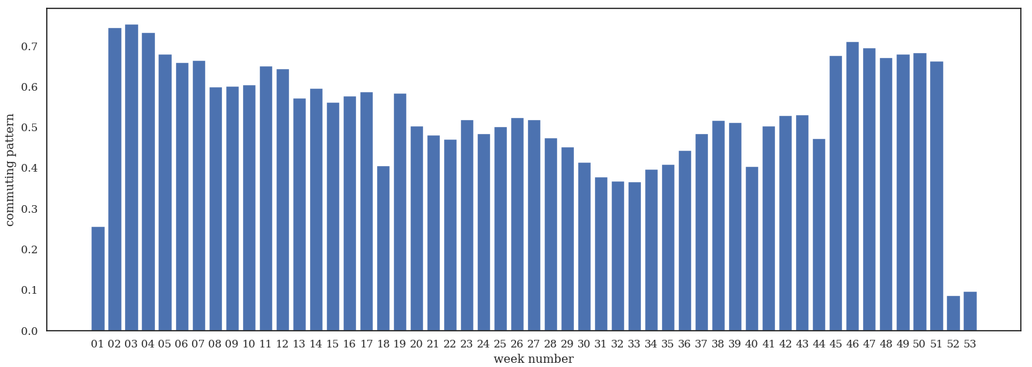 commuting pattern strength through all
locations
To compute a common year we build an isocalendar which is the representation of a year into
We worked to tune the network to avoid the system to fall in a local minimum
 training is trapped in a local minimum
This local minimum will turn to be the most common cluster which indeed has a good score with all other time series
 problems caused by boundary
conditions
We work on the dimension of convoluting filters to obtain indentation (the flat daily profile is not strongly penalized).
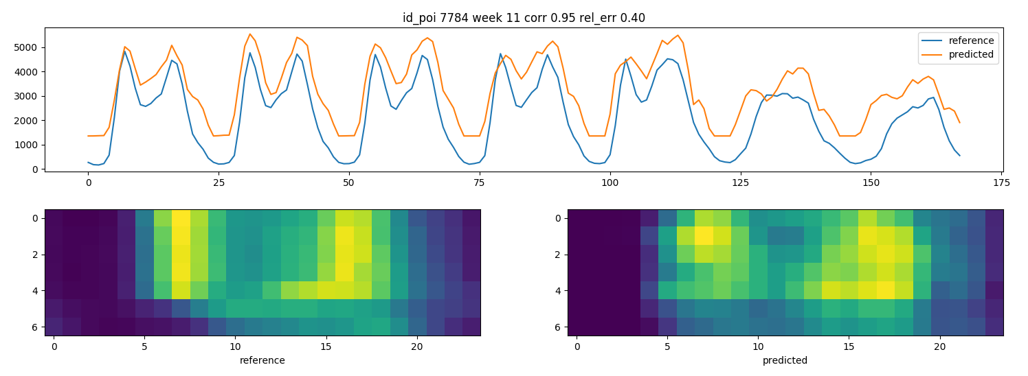 indentation
starts to appear
What happens if we upscale the image to have a larger dimension of images and we define a more complex network.
 upscaling a time series
Running time is drammatically increased but the convergence is not better.
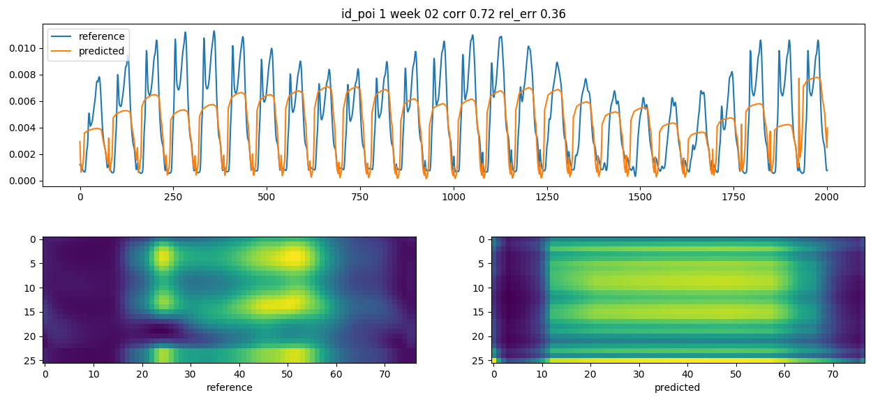 results of the upscaled time
series
The upsampling is not adding any useful information that the convolution wouldn’t We downscale the image and the result suffer from the same
 results of the upscaled time
series
In this case we remove the padding, cropping and up-sampling. We can see that in early stages the boundary has a big effect in prediction.
 morphing for flat convolution, earlier
steps
We can see that the prediction is really close to the reference series
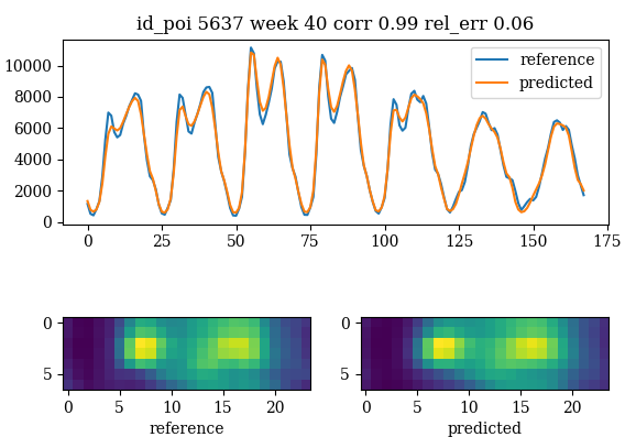 prediction for flat convolution
We realized as well that the model is drammatically overfitted.
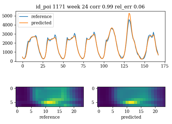 overfitted model
We reduce the number of parameters to try to capture the most essential feature of a weekly time series downscaling the image with a 3x3 pooling.
We see the modification of the external data into the model trained for the motorway counts.
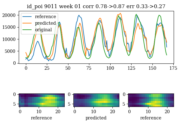 prediction using a short
autoencoder
Some times even the short convNet look like overfitting
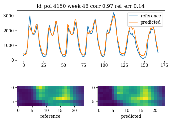 The prediction in limiting cases look
overfitting
In case of a picture we would have 7x24x256 = 43k values to predict, if we downscale from 8 to 6 bits we still have 10k parameters to predict. The dataset has a lot of redundancy and we should size the model to not consider too many parameters to avoid overfitting.
| method | params | score auto | score ext |
|---|---|---|---|
| max | 43k | ||
| interp | 12k | ||
| convFlat | 2k4 | ||
| shortConv | 1k3 |
To select the appropriate via nodes we run a mongo query to download all the nodes close to reference point. We calulate the orientation and the chirality of the nodes and we sort the nodes by street class importance. For each reference point we associate two via nodes with opposite chirality.
We can see that the determination of the via nodes is much more precise that the tile selection.
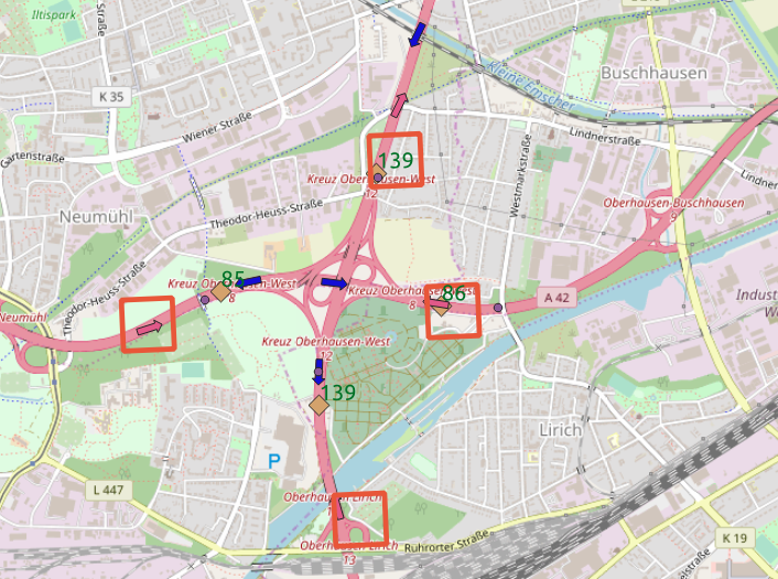 identification
of via nodes, two opposite chiralities per reference point
The difference is particular relevant at junctions
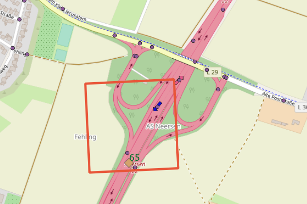 via nodes on junctions, via nodes do not count
traffic from ramps
Once we have found the best performing model we can morph our input data into the reference data we need. We have two sources of data which similarly deviate from the reference data.
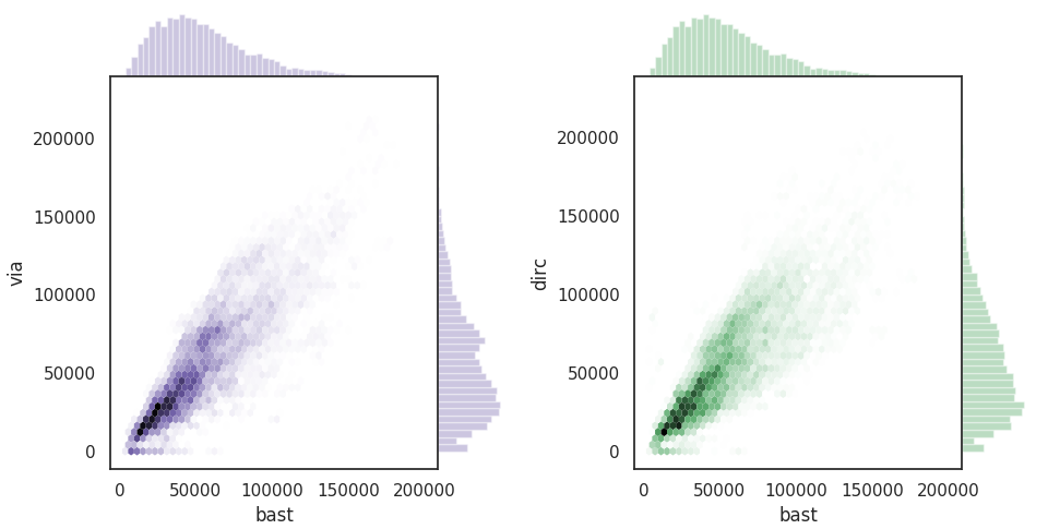 distribution of via and tile counts compared to BaSt
We first take the flat model and we see some good
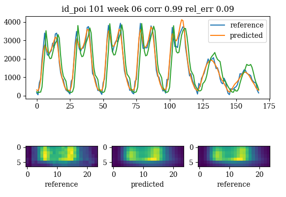 prediction from external data
The model is good for denoising spikes in the source
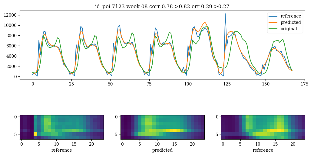 denoising functionality of the model
We don’t see a strong improvement in performances due to the overfitting of the flat autoencoder.
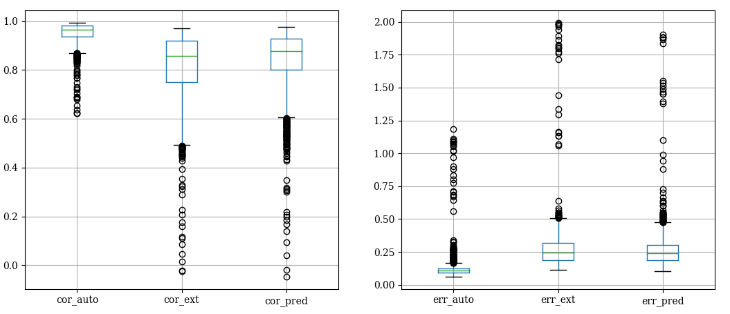 drop in performances applying the autoencoder
on external data
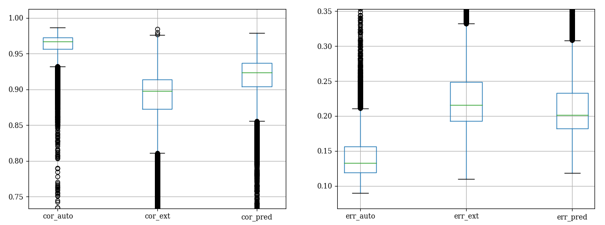 we have good performances with the short
autoencoder that avoids overfitting
If we need to write a source dependent model we use the same network to predict from internal data the reference data.
The encoder helps to adjust the levels especially for daily values
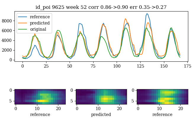 prediction with the encoder
The encoder helps as well to reproduce the friday effect
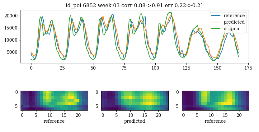 prediction has a better friday
effect
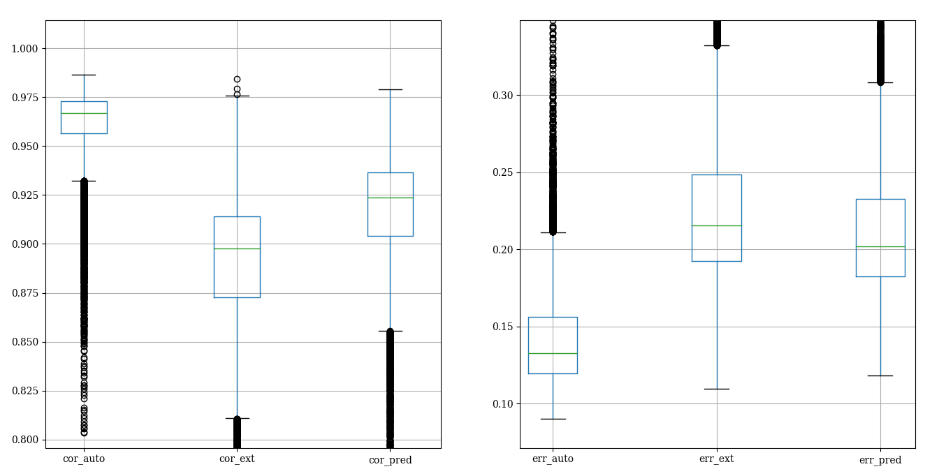 the encoder increases performances but the
original data already score good performances
