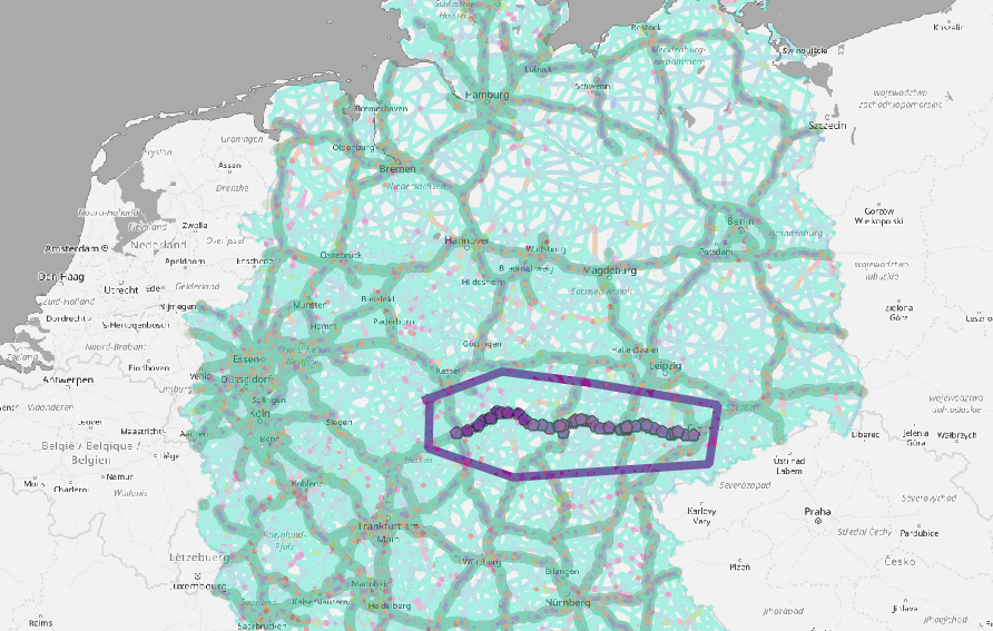
 selected
motorway stretch
selected
motorway stretchIn this project the attention is to know the distribution of cars entering and exiting the motorway.
We have tried different approaches to solve the problem and we have defined some KPIs to have a quantitative evaluation of the perfomances of each model.
The focus of this project is to understand where motorway drivers enter and exit a particular junction of a motorway as described in this ticket.
The overview of the parquet files is used to compare the different analyzer runs.
We have selected 12 junctions on a isolated motorway (A4) crossing Germany on the east-west axis.
 selected
motorway stretch
Chains from the tripEx are filtered via a pre validation script.
We try to obtain the same information on tile counts. For each junction we have to correctly report the incoming and outcoming flux.
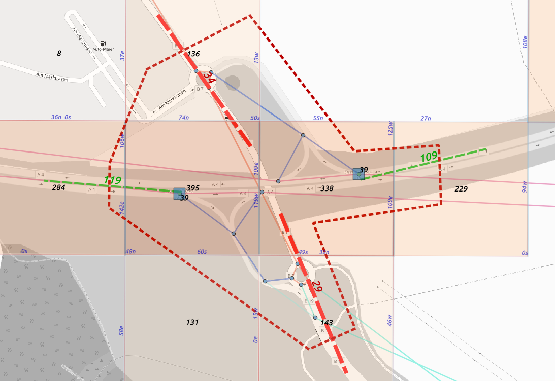 counts across tiles
We keep junctions in the network which are labelled differently from the other street classes.
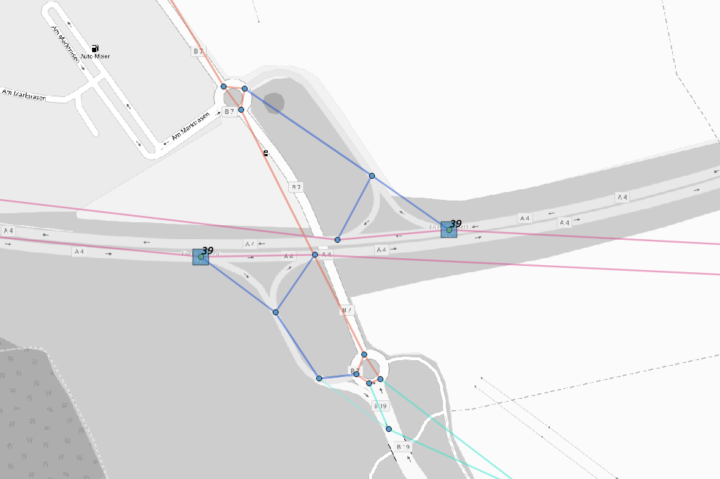 junctions into network
local motorway structure
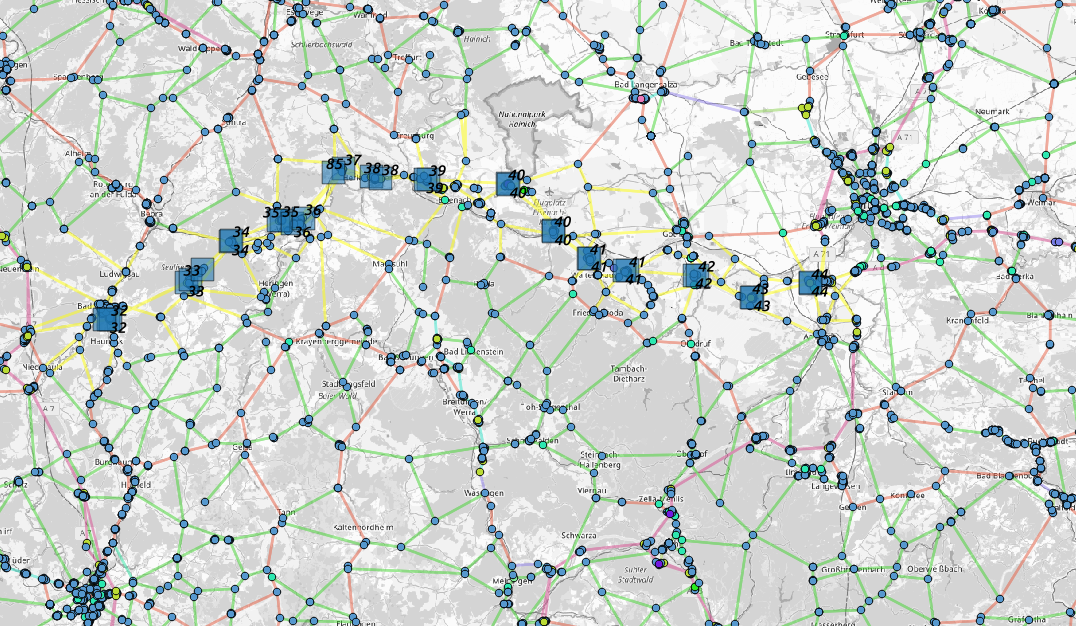 local motorway structure
routing, wrong weighting
We worked at the correct weighting between highway classes: 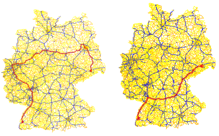 routing, improve in weighting
empirical definition of weights that led to qualitative good routing solutions.
if edge[2]['highway']=='motorway':
    attrs['weight'] = edge[2]['length']*1
elif edge[2]['highway']=='primary':
    attrs['weight'] = edge[2]['length']*1.5
elif edge[2]['highway']=='secondary':
    attrs['weight'] = edge[2]['length']*1.8
else:
attrs['weight'] = edge[2]['length']*3We took a random node for each zip code and we calculate the shortest route between each other zip code zip2zip.
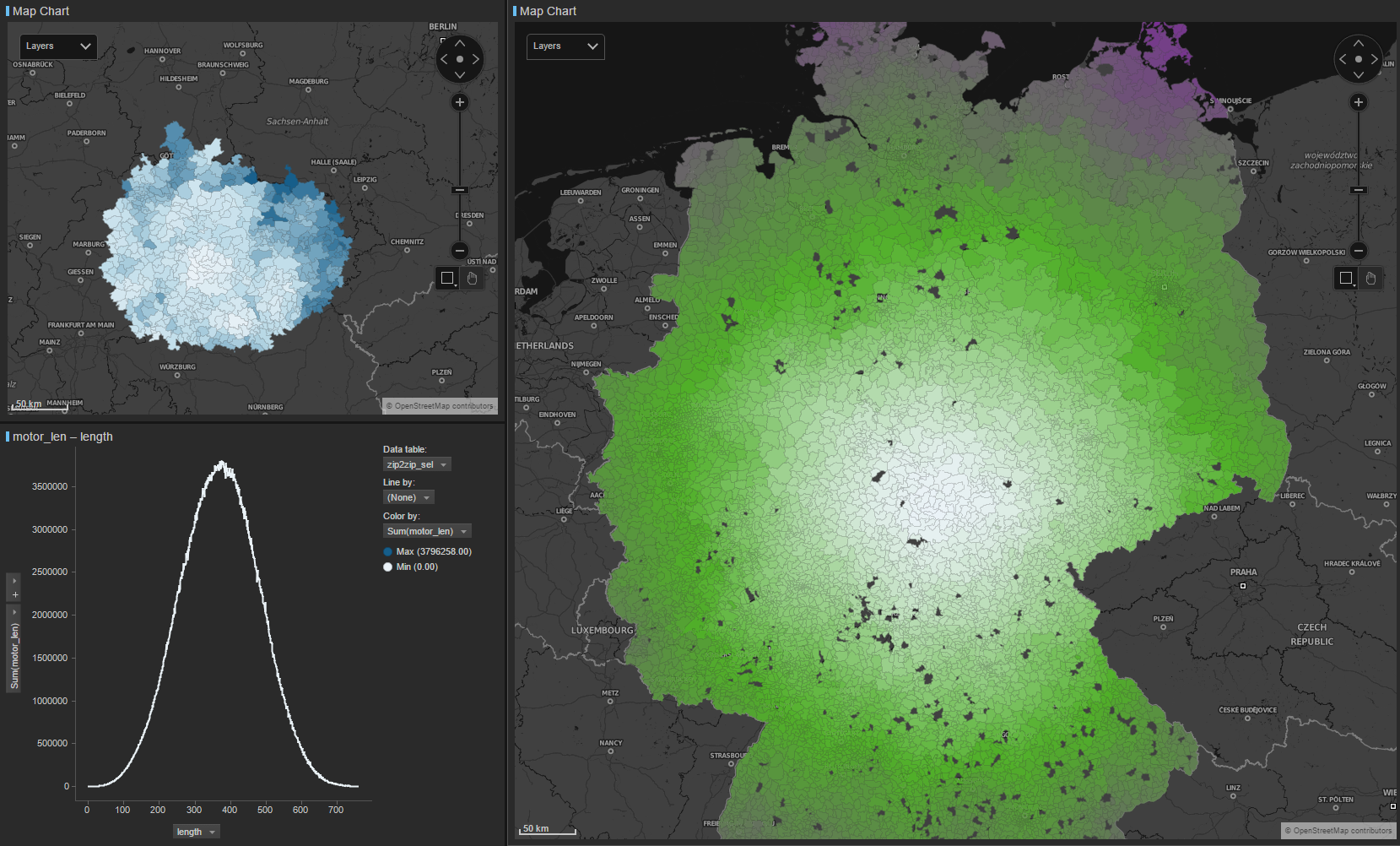 zip 2 zip distances
For each zip2zip relation we identified the first and last junction crossed by the route.
we than processed an ODM between all zips in Germany for 9 days and we joined it with the precomputed zip2zip junction relation to count how many trips are probably routed via motorway junctions.
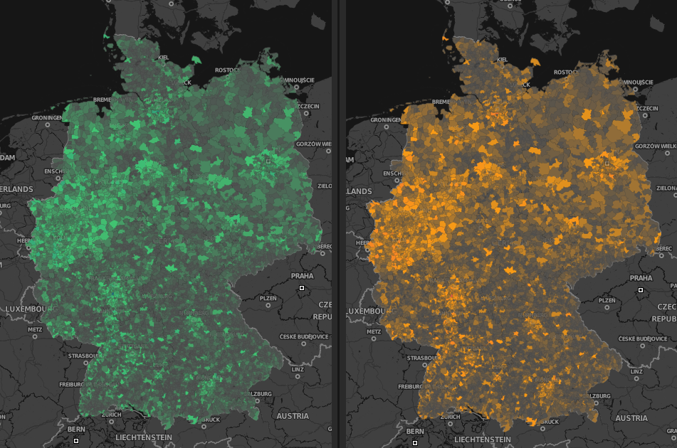 odm on 9 days
We run an ODM with a short and a long break parameter to see the difference in counts and understand where people could have a break on the way.
After iterating on all steps of the process, 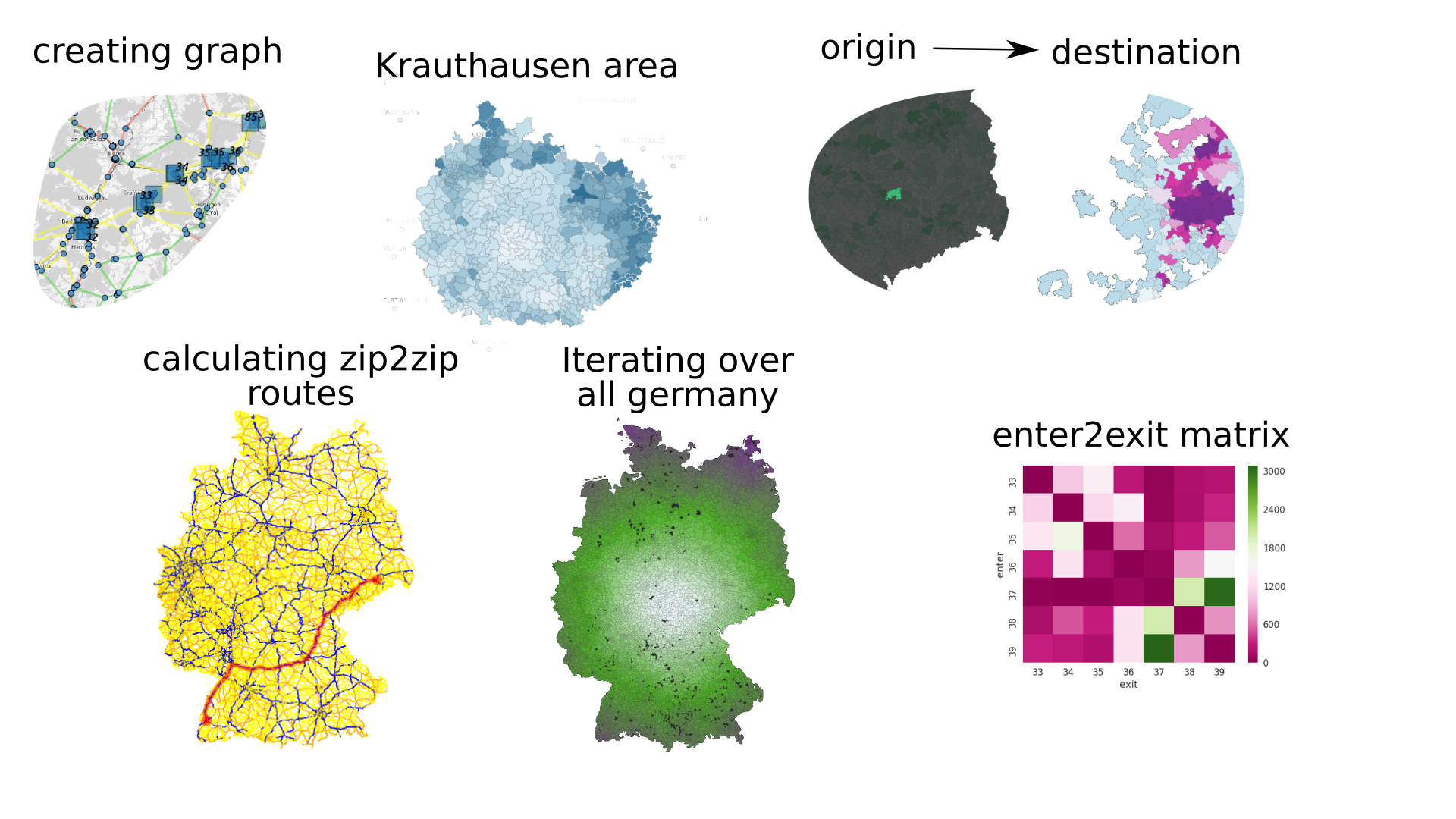
we have created the enter to exit relationship matrix.
 enter2exit via postprocessing
We realized with an ODM via that the counts of people leaving the
motorway wasn’t consistent and we couldn’t fix the unbalance between
junctions in post processing. 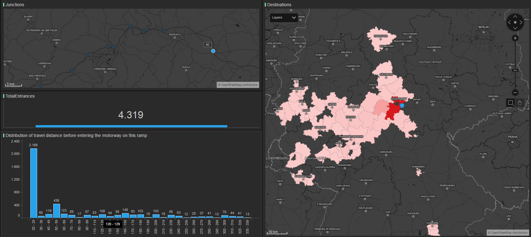 In post processing we filtered out fuzzy
relations caused by detours
We have manually added unique via nodes on the motorway links into our infrastructure
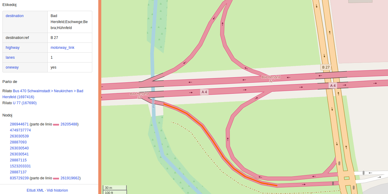 via point on
junction
We associate this points to a location and we group entrances and exits together:
 "input_locations":[
      {"location_id":"exit_32",
        "node_list":[263030540, 2675499063]},
      {"location_id":"entry_32",
        "node_list":[227910516, 25418734]},
and created the appropriate qsm job where all nodes are grouped into via locations.
These chains are passed thought the analyzer and we analyze a few trajectories.
At first we spot some strange behaviour:
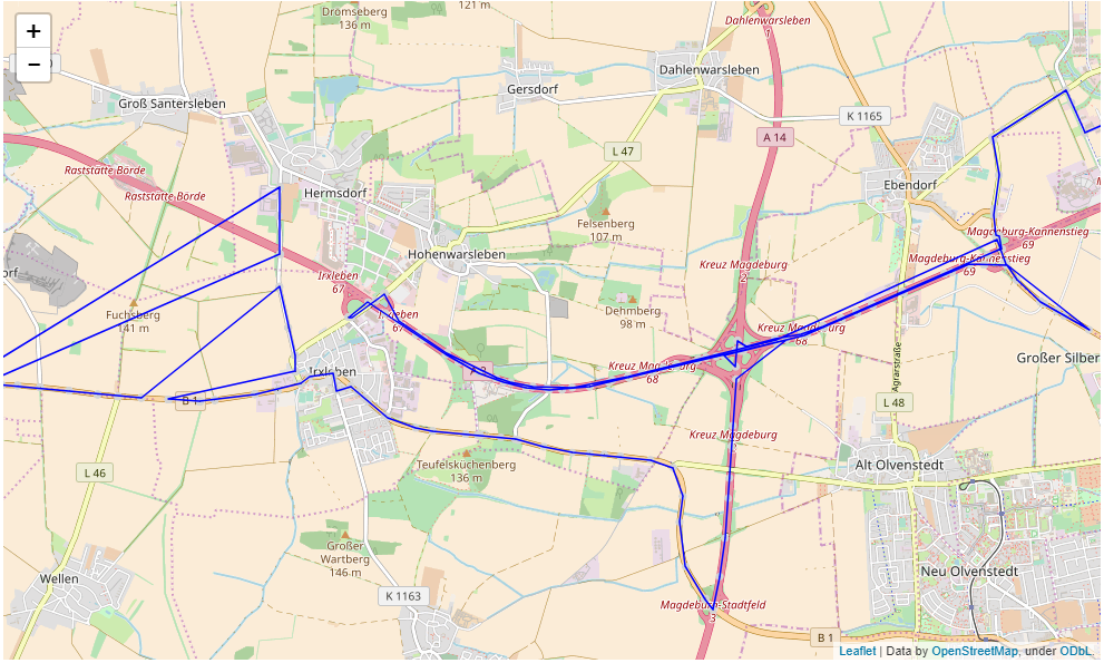 inspection on routing
After the second analyzer run:
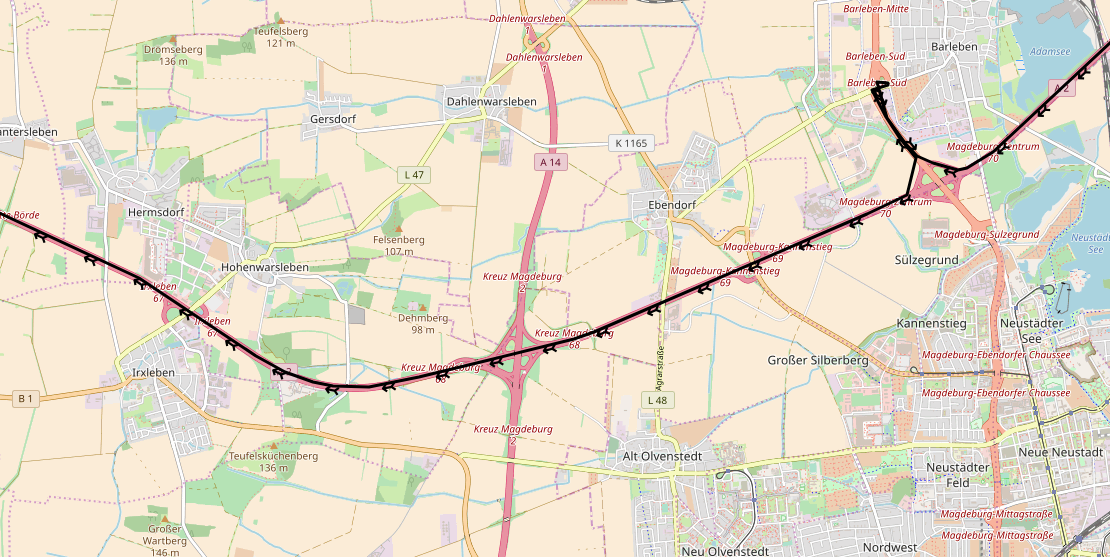 inspection on routing, second run, improved
results
We analyze the number of users passing by entrances and exits and find the relationships between ramps: via counts, traffic on some via nodes
We look at the size of entrances and exits to spot possible
asymmetries:  The
radius show the size of entrances (blue) and exits (red), circles are
pretty symmetric
We investigated the relationship between via nodes on the junctions and we spot some detours that falsify the counts that we are going to correct in postprocessing.
We visualize some relationships using kepler
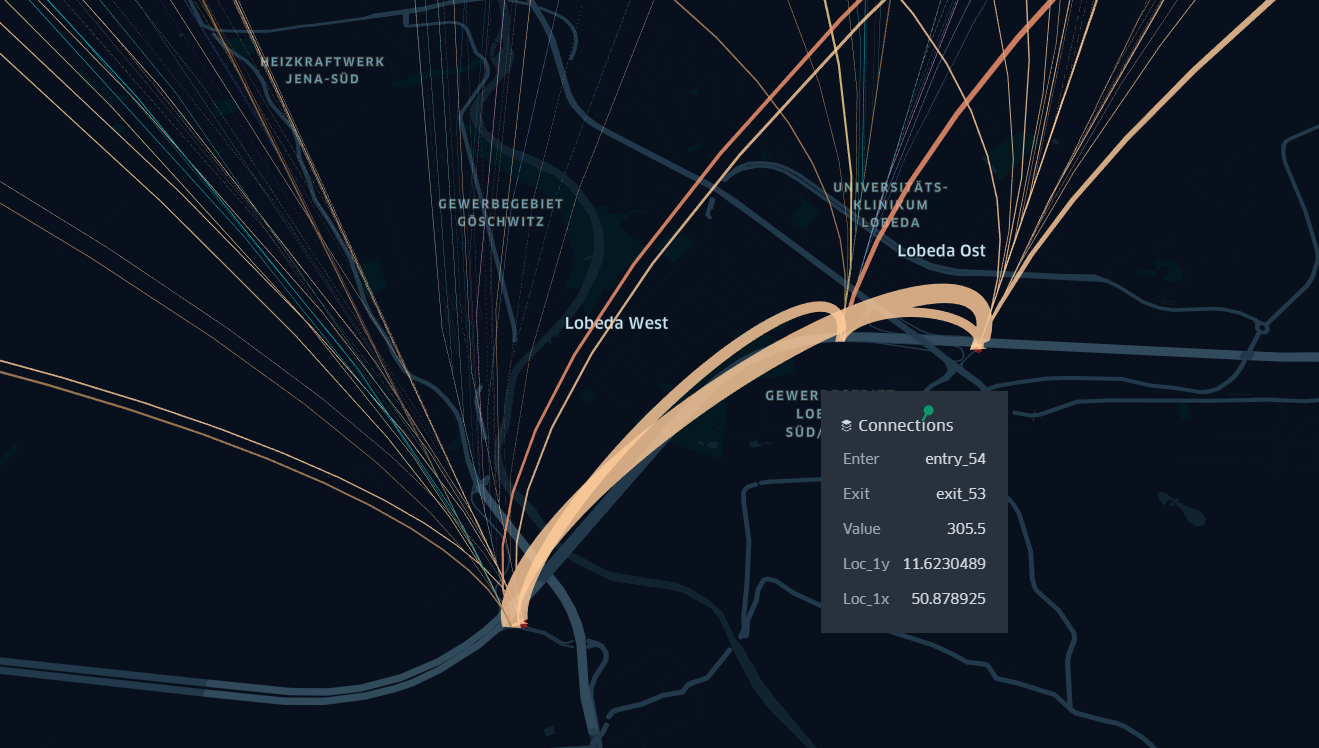 visulization of pair relationships
We consider the first entrance and the last exit removing all internal loops etl_nissanVia
exit_36;entry_36;exit_41b;entry_42 -> entry_36;exit_41b
exit_34;entry_34;exit_36;entry_40b;exit_41a -> entry_34;exit_41a
This filters out 26% of all trajectories which have no 1st entry and lst exit.
We remove unrealistic routes:
entry_56a;entry_41b
exit_32;exit_42;entry_42
We keep strange routes:
entry_59, exit_61, entry_60, exit_57In this way we can build a matrix of all the connections between
junctions.  We count
all the pair connection between junctions, we see how connections get
thinner on larger distances
We pivot the table and obtain a square matrix showing all the enter and exit relations:
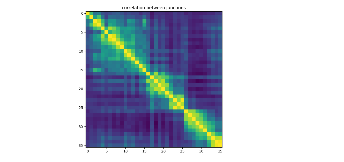 correlation between junctions, neighboring junctions show good
correlation, we must investigate the boundaries of the correlation
blocks
To obtain the routed distance between junctions we request an openstreetmap api.
    baseUrl = "https://api.openrouteservice.org/directions?"
    nodeD = []
    for i in range(nodeEn.shape[0]):
        for j in range(i+1,nodeEx.shape[0]):
            g1 = nodeEn.iloc[i]
            g2 = nodeEx.iloc[j]
            print("%s - %s : %.2f%%" % (g1['loc'],g2['loc'],(i*j)/(nodeEn.shape[0]*nodeEx.shape[0])))
            queryS = "api_key=" + cred['openroute']['token']
            queryS += "&coordinates="+str(g1['x'])+"%2C"+str(g1['y'])+"%7C"+str(g2['x'])+"%2C"+str(g2['y'])
All junctions over 150km from a reference junction are labelled as 996 because the current autonomy of the electric car under study is around 160km.
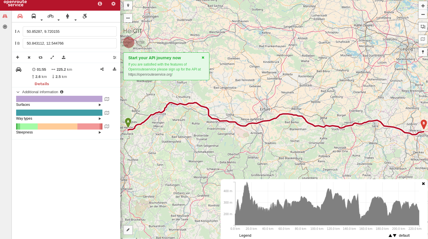 we use openrouteservice to calculate distances
between junctions
The expected output of the enter2exit matrix should have the expected properties:
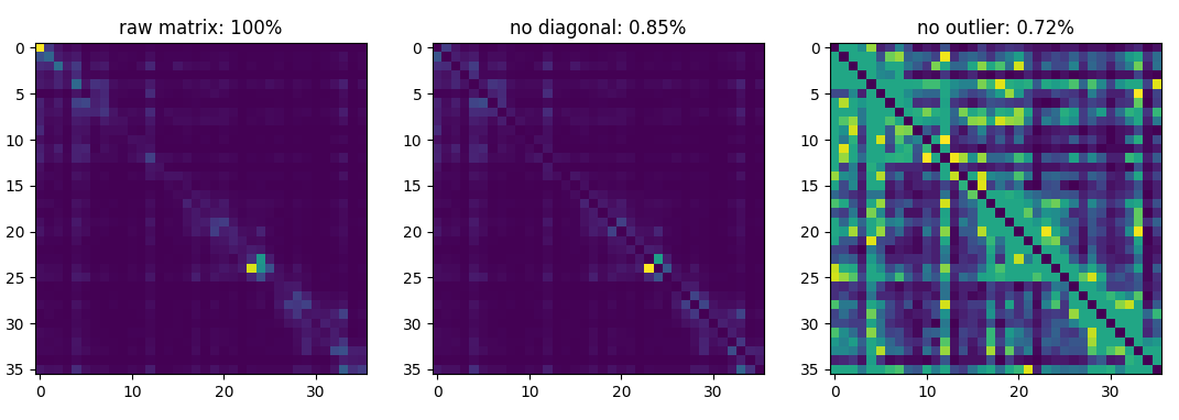 the enter2exit matrix has diagonal counts:
13% and outliers: 5%.
| KPI | single | clamp |
|---|---|---|
| diagonal | 15% | 26% |
| asymmetry | 26% | 21% |
| decay - correlation | -0.3 | -0.4 |
We display the asymmetry matrix coloring all cells under 10% relative difference with green, all cells between 10% and 20% with yellow and over 20% with red.
We have clamped the odd numbered juntions into the even ones.
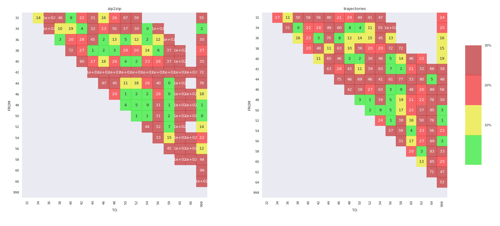 asymmetry matrix with traffic light color code,
we compare postprocessing approach (left) with single trajectory sum
(right)
$$ \delta = 2\frac{|c_{AB} - c_{BA}|}{c_{AB}+c_{BA}}\cdot w(m_{AB}) $$
where cAB is the number of cars going from A to B
$$ w(m_{AB}) = b + m_{AB}\frac{1 - b}{max(m_{AB})} $$
and mAB is the maximum between cAB and cBA and w is the weighting function and b the intercept.
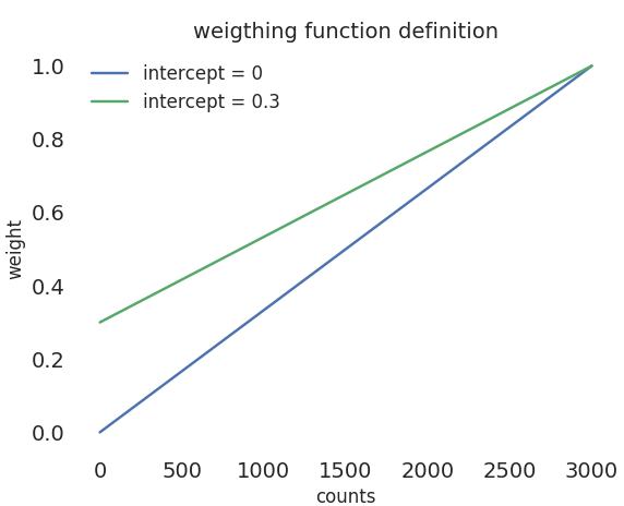 definition of the weighting function
| range | trajectories | zip2zip |
|---|---|---|
| within 10% | 39% | 24% |
| within 20% | 26% | 12% |
| over 20% | 35% | 64% |
We see a small dependency between junction length and number of cars.
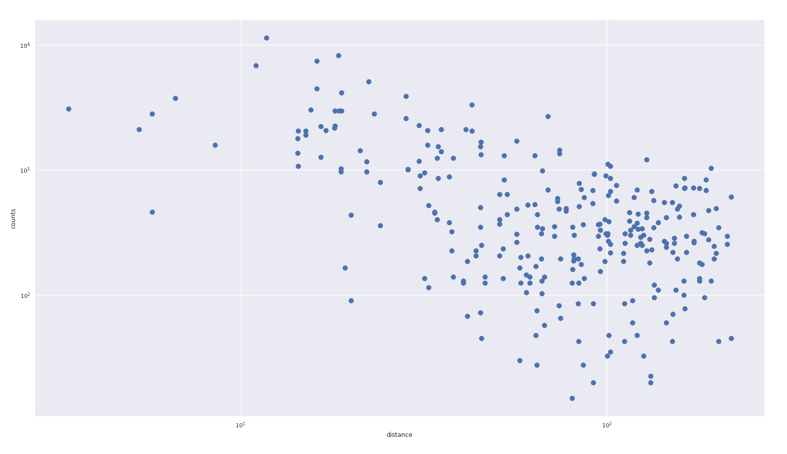 the number of cars decay with junction
distance
We have realized that some junctions were particularly asymmetric and we started investigating few trajectories
We saw some trajectories be forced to take the junctions
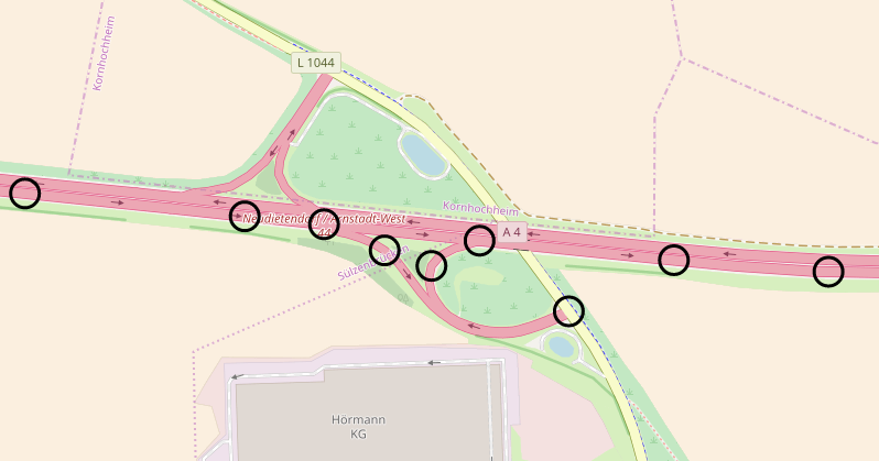 some routes
are forced to proceed on the junction
We sorted the timestamps and saw a strange arrangements of nodes.
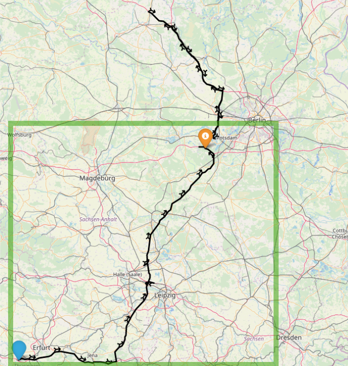
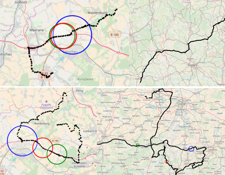 start (green) end (red) and junction (blue) are
not conseguent
We saw that an unprecise definition of the starting point led to detours.
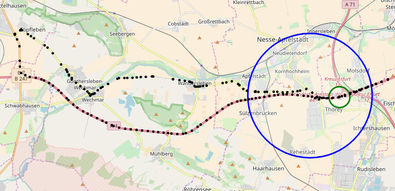 the start node competes with other events
that might help to distinguish the real start
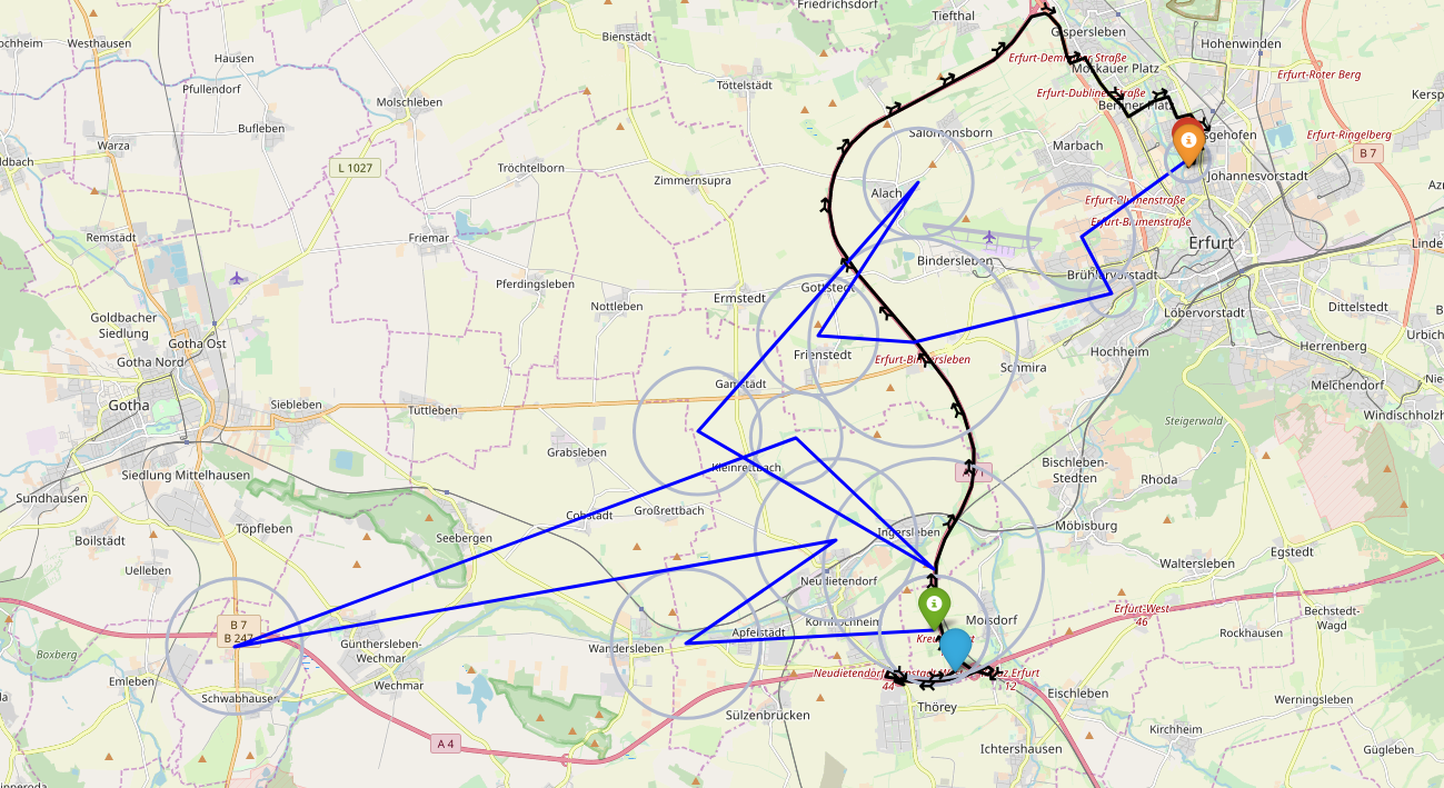
B-spline are important to neutralize the swing between cities that are denser in cells which force the trajectory to leave the motorway to approach to a city and go back to continue the trip.
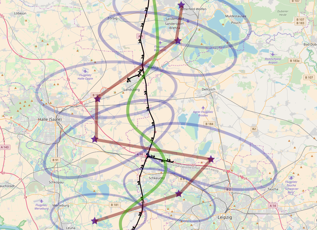 black: routed trajectory, red: events
line, stars: hypothetical cell’s centroids, ellipses: hypothetical BSEs,
crossing the motorway
There are different issues (routing, starting-ending point, graph) from my opinion:
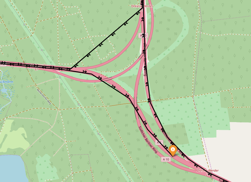 starts and ends on the motorway lead to
asymmetry
My suggestion is to update our graph to have a series of parameter which can help the routing:
When we transform the complete OSM node collection into our production graph I would add the following attribute to each segments of graph:
 enter and
exit bounding box
 detours bring to asymmetry
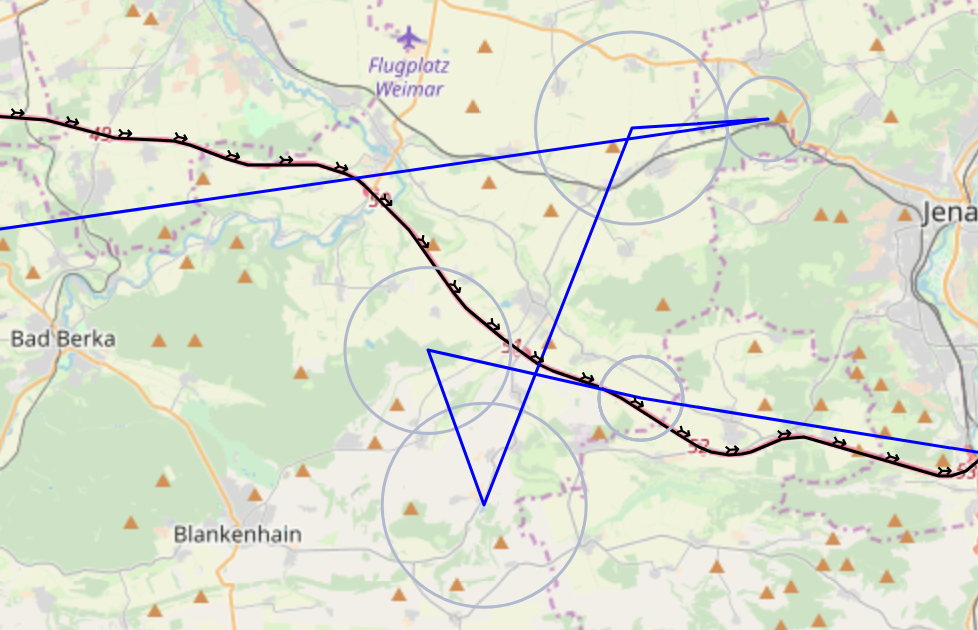
To avoid detours we have started using AB routing which drammatically improves the number of loops.
 AB routing avoid detours
 detour avoided discarding neighboring
events
The series of iterations we did helped improving the precision of the
enter2exit relations. The last run consists on a more days sum. 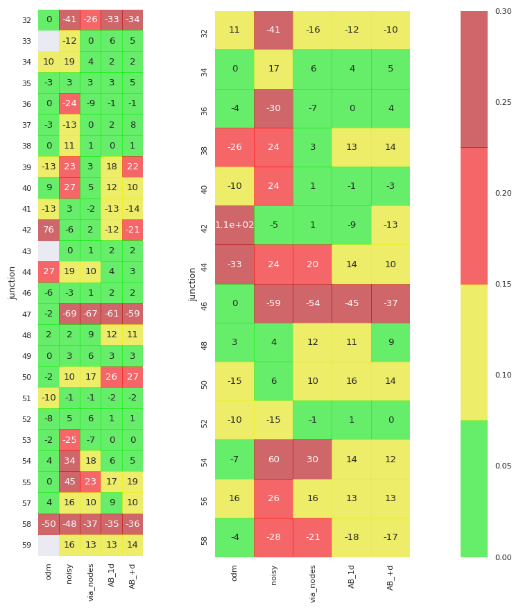
The asymmetry matrix view show how the precision of the asymmetry
improved from the first to the last analysis. 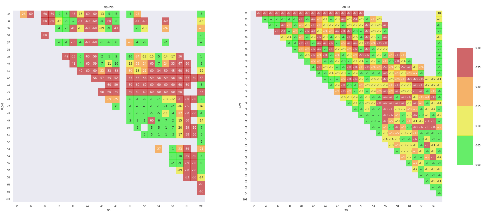
We still can see few problems to solve:
To automize the labelling of the nodes of the junctions we write two functions.
id_jun, chi,
id_zone, and dir to calculate the local center
of mass and the orientation depending on the cross product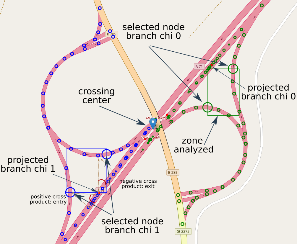 graphical
explanation on the selection and identification of nodes works
The algorithm supposes there are two branches per motorway and one entry and one exit per branch. Everything is splitted in 700m cluster to improve the accuracy if the crossing is large enough.
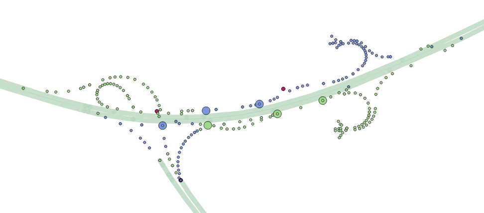 not all
topologies can be covered by the algorithm
After have labelled all junction nodes to be included in the infrastructure we run an odm any via for 1M3 chains dataset to obtain the number of trajectory crossing the via points in Thüringen.
We run the kpi calculation based on the results of the data
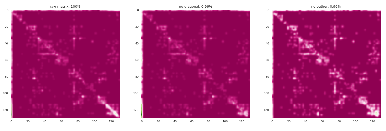 count matrices between entry and
exits
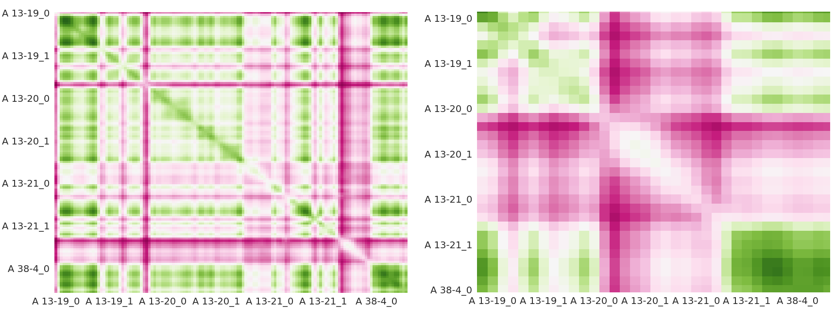 correlation
between pair relation counts, on the rhs we magnified the zone with
lower correlation
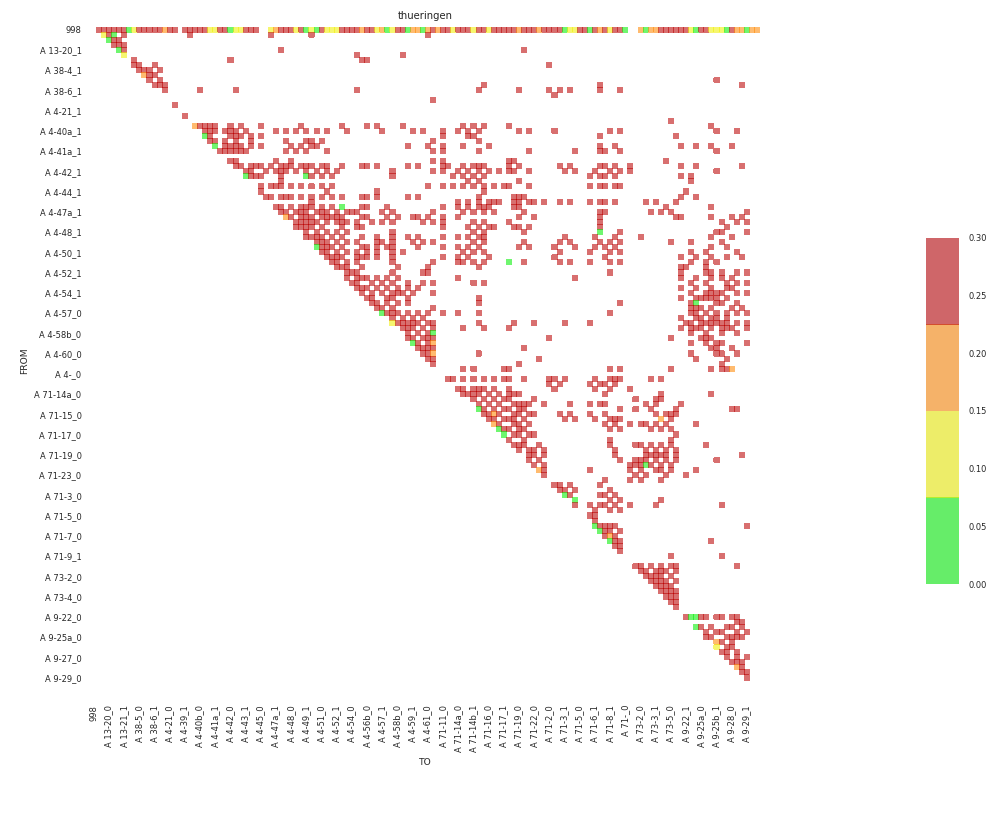 most of the relations show asymmetry but it’s
due to low counts
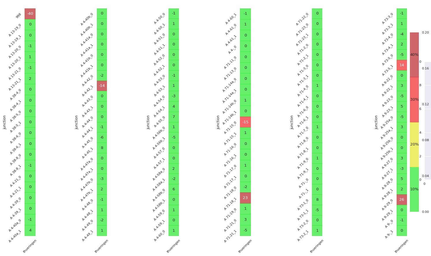 even on junction sum symmetry is not
conserved
No clear picture about result performances can be given with this few trajectories.
We perform a further correction of the job file and change the definition of the delooper. We break all the trajectories into single pairs. For every uncomplete entry or exit we associate the junction 998.
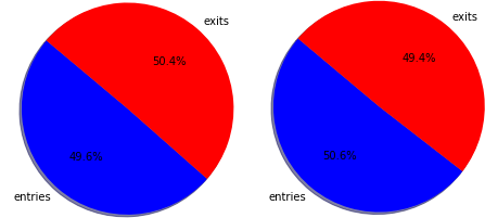 if we count the
total number of entrances and exits symmetry is conserved, both for all
the any via combinations (lhs) and for the 2 via nodes trajectories
(rhs)
We have a fair number of motorway junction crossed during a trajectory in Thüringen. 3 and 4 via node trajectories correspond to shortcuts, U turns and breaks.
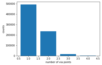 via points
pro trajectory
We than see that we still have asymmetries on the single junction
level but the total asymmetry is conserved 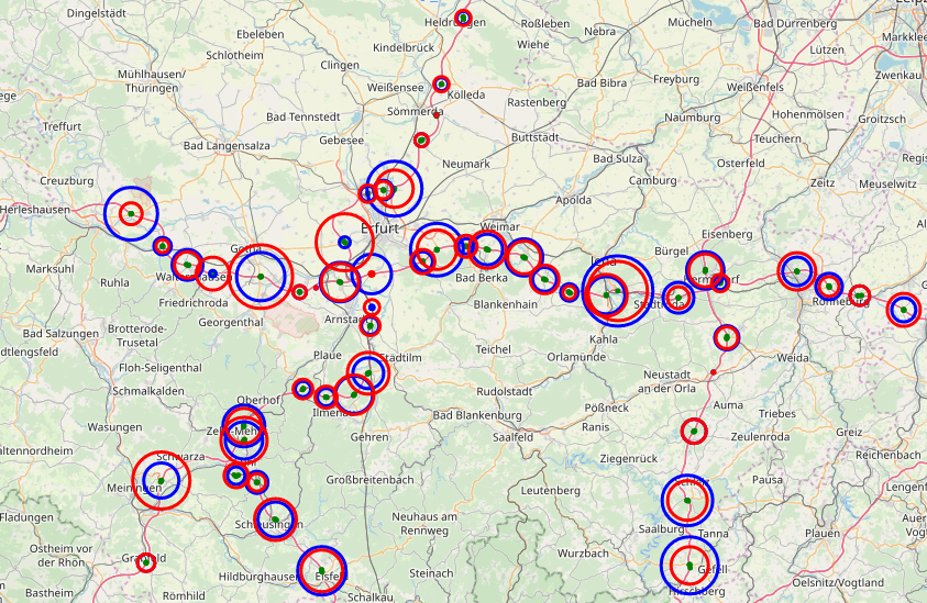 counts
of entries (blue) and exits (red) pro junction
