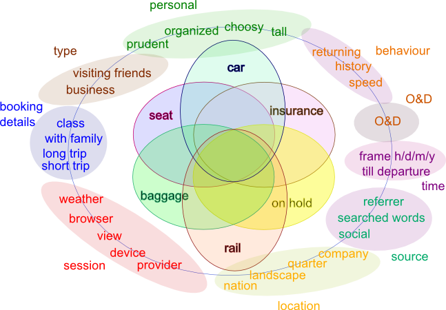
 Environement parameters and ancillary
offers.
Environement parameters and ancillary
offers.Data structure for real time parallel customer profiliation. Pretargeting, offer optimization, data structure, segmentation.
During a web session the parameters, pi, which can be
used for segmenting the audience are:  Environement parameters and ancillary
offers.
A learning process can be done correlating the performance of each teaser with the presence of a certain variable, e.g. via a naïve Baysian approach: $$ P(t|p_1,p_2,p_3,\ldots) = \frac{P(t)P(p_1|t)P(p_2|t)P(p_3|t)\ldots}{P(p_1,p_2,p_3,\ldots)} $$ Where P(t|p1,p2,p3,…) is the a posteriori probability of a teaser performance for a given presence of the paramters pi.
Since the number of parameters is around 1000/2000 this process is very inefficient and requires a large learning phase. Most of the environmental variables are correlated and should be hence clamped into macro environemental variables findinf the few functions that define an efficient session scoring. A big correlation matrix between all parameters should create a comprehensive hit map to guide the simplification and dimensional reduction of the parameter space. Second, some parameters shold be more influent in changing the teaser response and a correspondent ``learning weight’’ should be assigned to each parameter.
Offer performances should be tracked over different touchpoints to understand which options is the customer considering throughout his journey. Negative offer performances are as well really important to gain information about the customer.
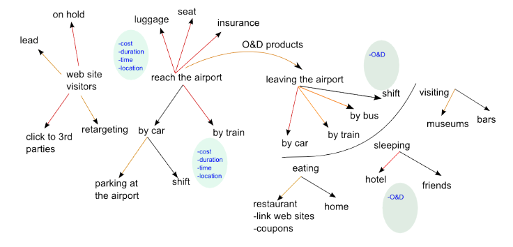 Customer journey, in red are listed
offered product, in orange potential product, in black alternative
decisions.
During a journey the customer has to take different decisions and decline an offer might be an important source of information about how he is confindent in the city he is visiting. For many biforcation points of his route we can consider a payoff matrix like: $$ \begin{array}{c c c} & disturbing & non-disturbing\\ available & a_{11}|b_{11} & a_{12}|b_{12}\\ non-available & a_{21}|b_{21} & a_{22}|b_{22}\\ \end{array} $$ Generally a11, a12, b12, b22 are negative. The determination of these parameters allow the estimation of a score about the customer/city link.
A set of semantic labels or categories (around 20) {l1, …, lNl}
that represent a target audience. Labels concern audience
whishes/interests and product properties, categories might be:
amusement, trend, luxus, tech, use At the beginning each ad is tagged
with a percentage of each label according to the opinion of the
marketer. 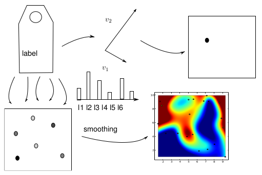 Up) representation of a label on the 2d plane. Down) collection of
all labels for ads and web sites and interpolated figure.
$$ a_1 = \{f_1l_1,\ldots,f_{N_l}l_{N_l}\} \qquad \sum_i^{N_l}f_i = 1 $$ The same is done for the web site according to the document analytic $$ w_1 = \{f_1l_1,\ldots,f_{N_l}l_{N_l}\} \qquad \sum_i^{N_l}f_i = 1 $$ Each label has a representation on a 2d plane, like arouse-valence plane (the 1d formulation is as well a good alternative). li = b1v1 + b2v2 b1, b2 < 1 The points might be alternatively regularly placed on a 2d grid. For each ad and web page we create a mask fitting the points with a Gaussian function.
The mask is the central concept of this method, it consists in 20-30
3d points (x,y,z) that are
interpolated via a 2d Gaussian. The mask might include in total 100$$100
points but the essential information is stored in few tens. For each
mask i we integrate its
orthogonal values vxi = ∫xf(x,y)dxdy vyi = ∫yf(x,y)dxdy
We represent all the masks as points on a 2d plane and perform a
Delauney triangulation (no need to calculate correlation matrices,
highly parallel) to isolate clusters. Clusters can be detected via
expectation-maximization algorithm. 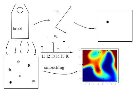 Representation of a mask on a 2d plane and
consequent clustering analysis on the data on the graph. Each cluster is
separated by a hull and for each cluster the average mask is
calculated.
For each cluster we calculate the average mask and a list of web pages or ads that belong to that cluster.
From each cookie we read the information about the web sites and the
ads clicked and create a user experience mask obtained by the sum of all
web and ad masks. 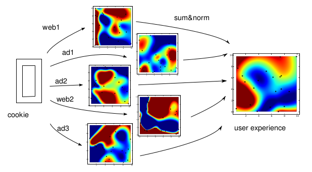 Creation of the user experience mask
as sum of ad and web relevance.
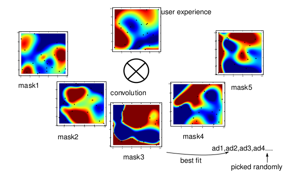
We perform a convolution with the cluster masks and select the best fitting opportunities. The best fit might be taken as well as the energy of the system, i.e. the energy closer to the largest value (Lx × Ly) is token. We show an ad on the web page currently viewed by the user by taking an ad randomly from the set of ads that belong to that mask. Each separated computing unit communicates the user experience matrix and the the user preferences to the central unit.
{"user":[
"id" : 10245,
"userexp":[],
"webuse":[],
"aduse":[]
]} melody
convolution
The computer unit stores information about the user
{"user":[
    "id" : 10245,
    "webvisited": [],
    "advisted": [],
    "adseen":[],
    "update":,
    "norm_weight":456732456
]}
The ``normweight’’, nw, number is used for normalization: if the next mask has weight 1 the former mask is multiplied by (nw+1)/nw while the adding mask by 1/nw.
The central unit computes all the user information assigning to each user experience matrix two vectors. Once the points are updated on the graph performs a cluster analysis and refine the web and ad masks. The new masks and ad lists are communicated to the external units after the calculation. Under convergence of points into separated clusters we perform coarse-graining of the information and we define each cluster as a hull. Each hull represents a different graph database to speed up the computation.
{"cluster":[
    "id" : 102,
    "hull_border": [],
    "u_mask": [],
    "db_address":,
]}
Each cluster can be separately processed.
Each external unit process the information about a single user with
no communication required among different units. 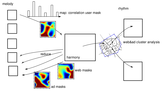 Structure of the different computing units and
the period segmentation. In the graph are shown the information during
the map and the reduce phase.
The central unit computes the masks and communicate the new values to each of the external unit in an asynchronous time. The external units are completely autonomous and the calculation time of the new masks do not affect the response time of the system. The masks can be time dependent and different sets of masks might be selected depending on the hour of the day or the day of the week.
Given: 50M users, 10G views, 1M url, 10k pages rCPO
10/order rCPC
1/click rCPM
1/1000views calc time 20ms, 50k calc/s. The calculations are meant to be
performed on the native machine via python or c++ code. The cookies are
text analysed after the last update, the masks relative to the visited
web site or ad are added to the user experience mask. During the update
phase the new user’s mask is mapped into the central unit and the new
information are updated in the graph. 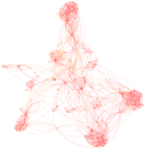 Typical graph database per 1M users (ref: pet
project.
According to the performances of Neo4j there should be no large computing time required to precess 50M nodes but different levels of coarse-graining might be introduced in the graph to improve performances. That means that different databases might be used to compute different magnification of the graph.
We know the ad visibility, the page visited and the ad selection.
 revenue figures
We construct the cumulative probability of the revenue summing up each single revenue $$ r_{tot} = \sum_i^3 f_ir_i \qquad i \in \{CPO,CPC,CPM\} $$ Where ri is the revenue of the offer and fi its frequency. We use a random number uniformly distributed, u, to select the offer $$ r_l = \frac{\sum_i^l f_ir_i}{r_{tot}} \qquad P(l|u) = P(u<r_{l-1} \& u\geq r_{l}) $$
To each ad, i, can be set a number that represents the distance of the ad mask to the average cluster mask, dci. The ad, instead of being selected with a random probability, might be selected using the cumulative probability of the sum of the distance from the center. $$ d_c = \sum_i^{N_{ad}}d_c^{i} \qquad d_c^l =\frac{\sum_i^{l}d_c^{i}}{d_c} \qquad P(l|u) = P(u<d_c^{l-1} \& u\geq d_c^{l}) $$ Where u is a random uniform number. ## Interest filtering
User grouping can be used to let new user filter information about
complex content in a web site.  Filtering dash based on user
grouping
The dash represents the same categories calculated by user grouping and let the user filter the information by populating the dash.
One of the scoring parameter for a customer is the analysis of the feedbacks he writes in different channels.
Specific customer feeedbacks were used to train dictionaries for the association of some keywords to specific arguments of sentiments.
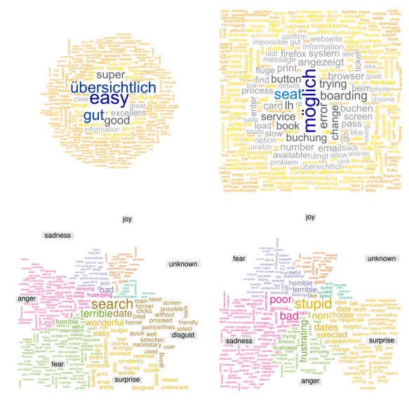 Training of dictionary for topic and sentiment
recognition.
The training of the dictionaries is really important for
understanding the sentiment of the customer and extract the most
relevant words. Those words can be connected to a particular
sentiment.
The customers were asked to choose a category and rate their
satisfaction to each comment. We had then the chance to create topic and
sentiment specific dictionaries to be able to automatic guess by user
input the most probable reason of his feedback. We run an emotion
recognition to understand which words are more common to different
topics.
 Distribution of sentence length, statistical
communality between months.
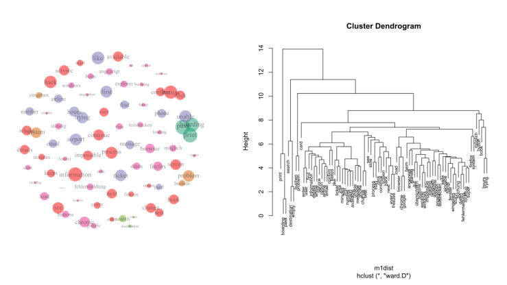
We have analyzed as well the clustering and the correlation between words to see whether it was necessary to clamp words together or to assign a cluster number to the words. It is as well important to read general statistical properties of the comment to recognize whether they are formally similar.
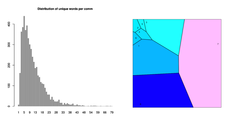 Distribution of sentence length, communality
between months, distribution of sentence length, statistical communality
between months.
In this case we can correlate time periods together to understand which topic are more interesting in particular time of the year.
Following the thermodynamic example the Gibbs free energy is:
G = U + PV − SΔT
if we want to translate this concept in terms of business we can say that revenue is the sum of the {} sold, the {} done and the {}. Sale has a major role the revenue that comes from the first two parts but a proper sale strategy can increase a significant gain in information. In the following we propose a sale oriented strategy with large focus on customer information gain.
 Sketch of the infrastructure and customer information flow.
Throughout this document we are going to analyze some branches of this sketch.
We consider a session as our variable x, for each session we can define a function g(x) that defines the revenue in the session. g(x) is defined as the sum of the acquired services, we define the ticket, t, as the main product and all other products, {a1, a2, a3, a4, …}, are ``attached’’ to the ticket. g(x) = wtft(x) + ∑i ∈ {a}wifi(x) where w is the margin for each sale and f the frequency of sale per session. We assume that the probability, p, of an ancillary sale is always conditioned by the ticket sale. $$ p_a := p(a|t) = \frac{p(a)p(t|a)}{p(t)}=\frac{p(a)}{p(t)} \qquad p(t|a) = 1 $$ where p is the probability correspondent to the frequency f. The metric m is the {} defined as the path to a {}. The straightes metric for the booking is: ProductList − ItemSelection − CustomerDetail − Payment The formulation of the ticket booking frequency ft is: ft = flist ⋅ fit ⋅ fcd ⋅ fbook where we call fst the frequency of a generic step conversion. When the booking comes from an external campaign an additional frequency is added: ft = (1−bouncerate) ⋅ flist ⋅ fit ⋅ fcd ⋅ fbook ## Variant testing If we split a page into different variants we influence the frequency of the conversion step: $$ f_{st} \to \left\{\begin{array}{c} f^a\\f^b\end{array}\right. $$ We perform a time average of the two frequencies, $\mean{f^a}_t$, $\mean{f^b}_t$ and find the winning variant performing a t-test $$ t_{test} = \frac{\mean{f^a}_t - \mean{f^b}_t}{\sqrt{s_a/N_a + s_b/N_b}} $$ Where Na and Nb are the sample sizes and sa and sb are the standard deviation of the correspondent frequencies and follow a χ2 distribution. If the difference between state a and state b consists in more than a single change we should consider the influence of each of the M element changes: $$ T^2 = \frac{N_aN_b}{N_a+N_b}(\bra{\bar a} - \bra{\bar b}) \mathrm{Cov}_{ab}^{-1}(\ket{\bar a} - \ket{\bar b}) $$ where Covab is the sample covariance matrix $$ \mathrm{Cov}_{ab} := \frac{1}{N_a+N_b-2} \sum_{i=1}^{N_a} \Big((\ket{a}_i - \ket{\bar a})(\bra{a}_i - \bra{\bar a}) + (\ket{b}_i - \ket{\bar b})(\bra{b}_i - \bra{\bar b})\Big) $$
The correspondent probability of a number of conversions, nc, in a day i, for an action xa, follows the Poisson distribution: (Γ(k) = (k−1)!) $$ p_{st}(n_c,t;\lambda) = \frac{(\lambda t)^{n_c}}{n_c!}e^{-(\lambda t)} $$ which is comparable to a Gaussian distribution with $\sigma = \sqrt{\lambda t}$ for λt ≥ 10.
The probability distribution of a data set {nc} is: $$ P_g(\{n_c\}) = \prod_{i=1}^N \frac1{\sqrt{2\pi n_i}}e^{-\frac{(n_i-\lambda_it_i)^2}{2n_c}} $$ The fitting parameter, λiti, can be determined by minimizing the χ2. $$ \chi^2 = \sum_{i=1}^{N_d}\frac{(n_i-\lambda_i t_i)^2}{n_i} $$ since for Poisson distributions σi2 = ni. If we instead measure a continous quantity attached to the action (e.g. price, xp) we can consider a Gaussian distribution $$ p_{st}(x_p) = \frac{1}{\sigma_p\sqrt{2\pi}} e^{-\frac{(x_p-\bar{x_p})}{2\sigma^2_p}} $$
We have defined the frequency of bookings ft as the product of frequencies per conversion step. $$ f_t = f_{list} f_{it} f_{cd} f_{book} = f_1 f_2 f_3 f_4 \qquad f_t \simeq f^0_t + \sum_{i=1}^4 tial_i f_t \cdot \Delta f_i $$ The error of the total conversion propagates as follow: $$ s_t^2 = \mean{f_t - \mean{f_t}}^2 = \sum_{i=1}^4 (tial_i f_t)^2 s_i^2 = f_t^2 \sum_{i=1}^4 (s_i^2/f_i^2) $$ Where we have assumed that cross correlations s12, s13, s14, … are all zero because of statistical independence of the different pages since no test is extended on another page. That implies that the less noisy metrics are short and defined across simple pages (few biforcation). The typical noise generated from a Poisson process is the shot noise, which is a white noise and it’s power spectrum depends on the intensity of the signal. The signal to noise ratio of a shot noise is $\mu/\sigma=\sqrt{N}$. To filter out the noise we have to study the autocorrelation function of the time series $$ corr_{f_t}(x) = \sum_{y=-\infty}^\infty f_t(y)f_t(y-x) \simeq f_0 e^{-cx} %\mathrm{or} f_0\left(1-\frac{x}{c}\right) $$ Being a white noise we can clean the signal removing the null component of the Fourier transform: $$ f_{clean}(x) = \int \left( \hat f(k) - \frac1\pi\int_\pi^\pi f(x) dx\right) e^{-2\pi\imath xk}dk $$ All the different variants of the tests (e.g. languages) should have a comparable power spectrum.
Another important parameter is the {} which can be defined as q(x) := q(x|Gp,Gw,Cl,Sp) Which is a function depending on the scores: * Gp Expenditure capability (maximum budget) * Gw Expenditure willingness (flexibility in acquiring services) * Np Network potential (influence on other travelers) * Cl Customer loyability (persistance in booking) * Sp Information Gain A possible definition of those quantities is: $$ G_p := max(g) \qquad G_w := \frac{|g_t - g_{tot}|}{g_{tot}} \qquad C_l := \frac{t_{x}}{\bar t}\frac{m_{x}}{\bar m} \qquad S_p := \sum_i p_i\log\frac1{p_i} $$ Where pi is the ratio between teaser conversion and teaser generation. Session quality is an important score for session
