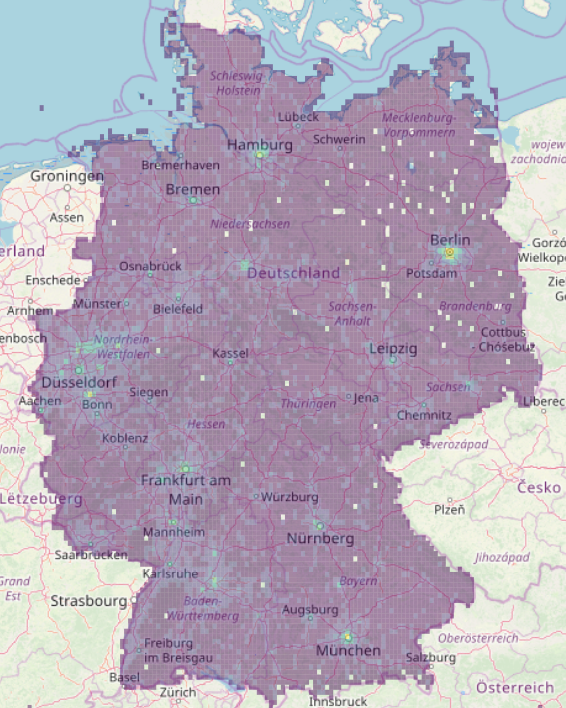
 density of gps events across germany
 density of gps events across germany
We get for each user a line with x and y coordinates, device type, accuracy in meters and time zone. For each coordinate pair we create an octree index for the given accuracy
| ts | id | type | x | y | accuracy | tz | octree | n |
|---|---|---|---|---|---|---|---|---|
| 1556146040 | 00002af79399fef8e… | 0 | 52.2833 | 7.93245 | 17 | 7200 | 314223124321441 | 1 |
From the positions we calculate the densities grouping by octrees and we remove one octree digit every time the number of events is smaller than a threshold.
In between we calculate the average position and time for each box.
| octree | n | x | y | ts |
|---|---|---|---|---|
| 422331313214 | 35 | 7.5405 | 47.712 | 1554083921 |
We can than convert the octrees in polygons and display the density values with a color map rendering first the large boxes.
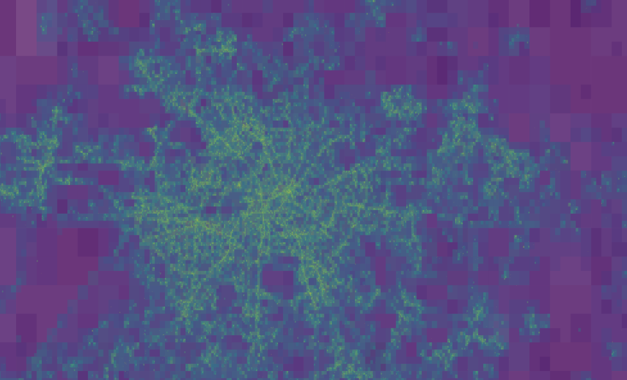 densities in the city
We can clearly distinguish users driving on main roads
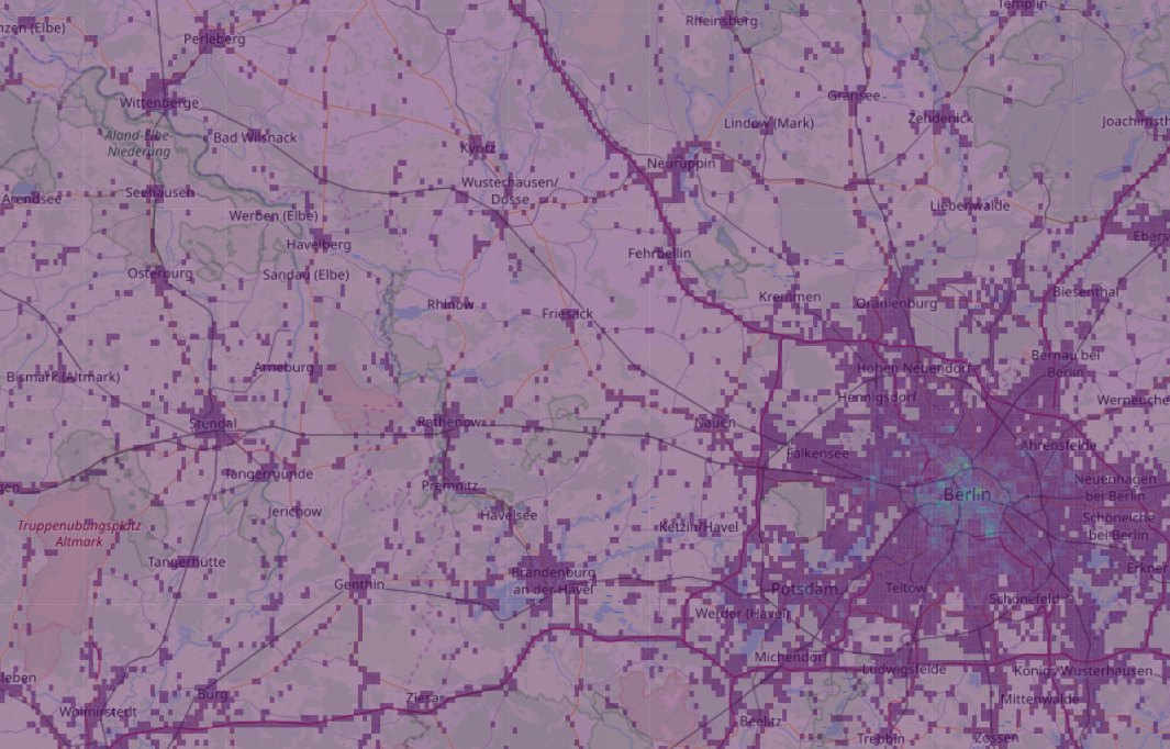 density on the streets
We pivot all entries by the user id and we create a new dataframe where on each line we have id, time-space matrix, n trajectory points, bounding box in octrees, time interval
| id | tx | n | bbox | dt |
|---|---|---|---|---|
| 933a58bfed63df92570… | [[1556210261, 13.497, 52.395], [155626... |
976 | 423 | 15562 |
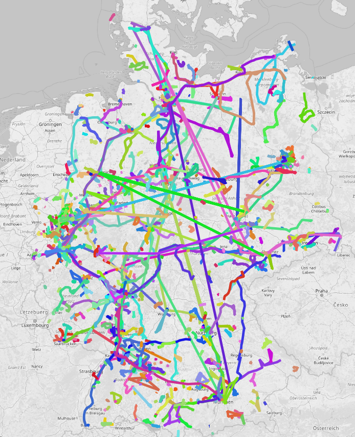 trajectory
country
All trajectories are defined by a bounding box which makes spatial filtering efficient
 densities and trajectories
We create a dataframe each day to know how many users we see in the country
| id | ts |
|---|---|
| 00002af79399fef8eb17522aedba3cedc45bb3cd193a34… | 85 |
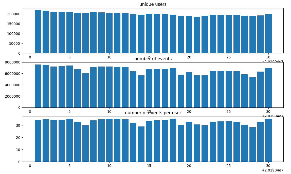 user frequency
If we look at the distribution of events per users we notice extreme numbers and the median drops to 19
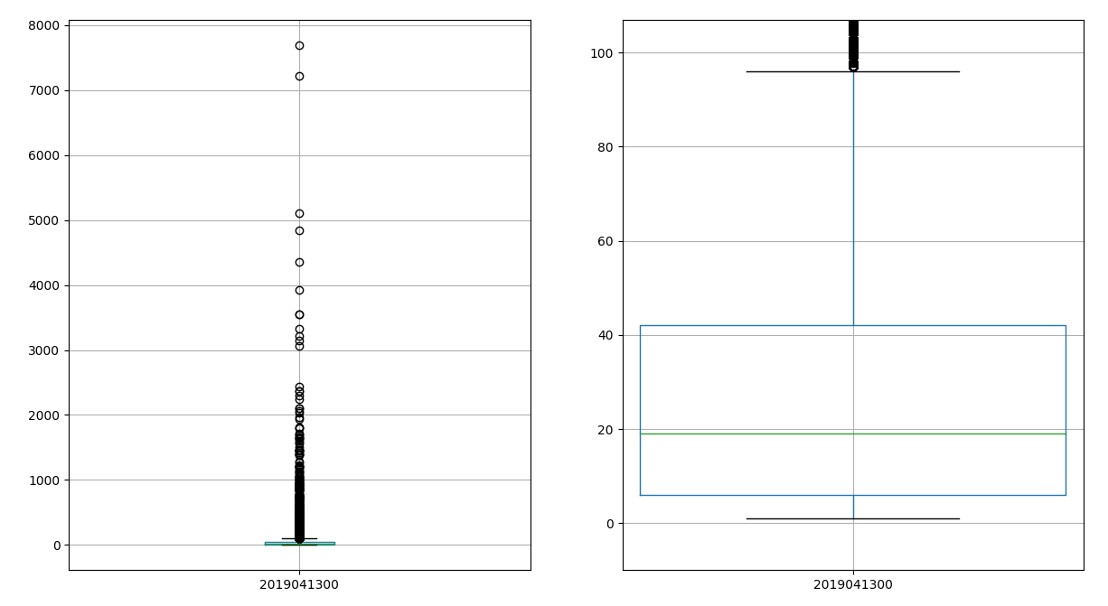 user distribution
We iterate over all trajectories and calculate the point to point space-time difference. We derive than the speed, the angle and the chirality of the segment.
| octree | n | speed | angle | chirality |
|---|---|---|---|---|
| 423144344341423 | 1.0 | 0.000008 | 0.957055 | 1.0 |
Where we calculate the speed as a normal equation of motion
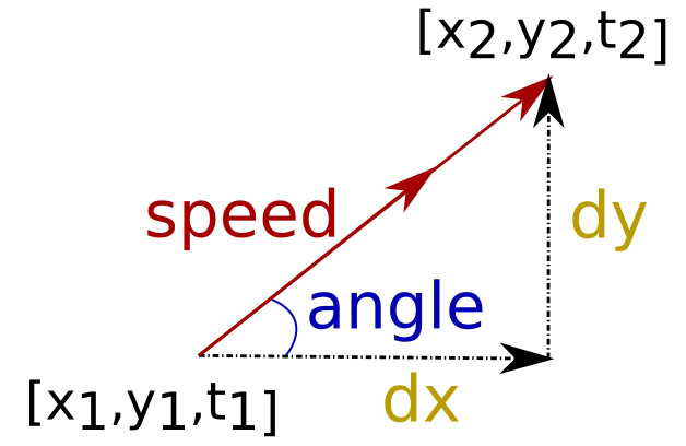 speed calculation
To calculate the segment speed we need first to smooth the input variables inducing correlation between the points. Without smoothing data are too noisy to be processed
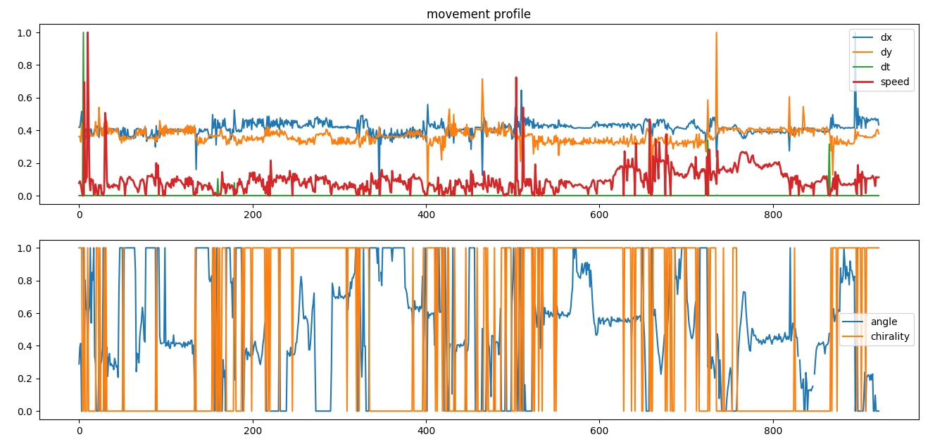 speed, no smoothing
If we use a running average space-time and their derivatives are better defined
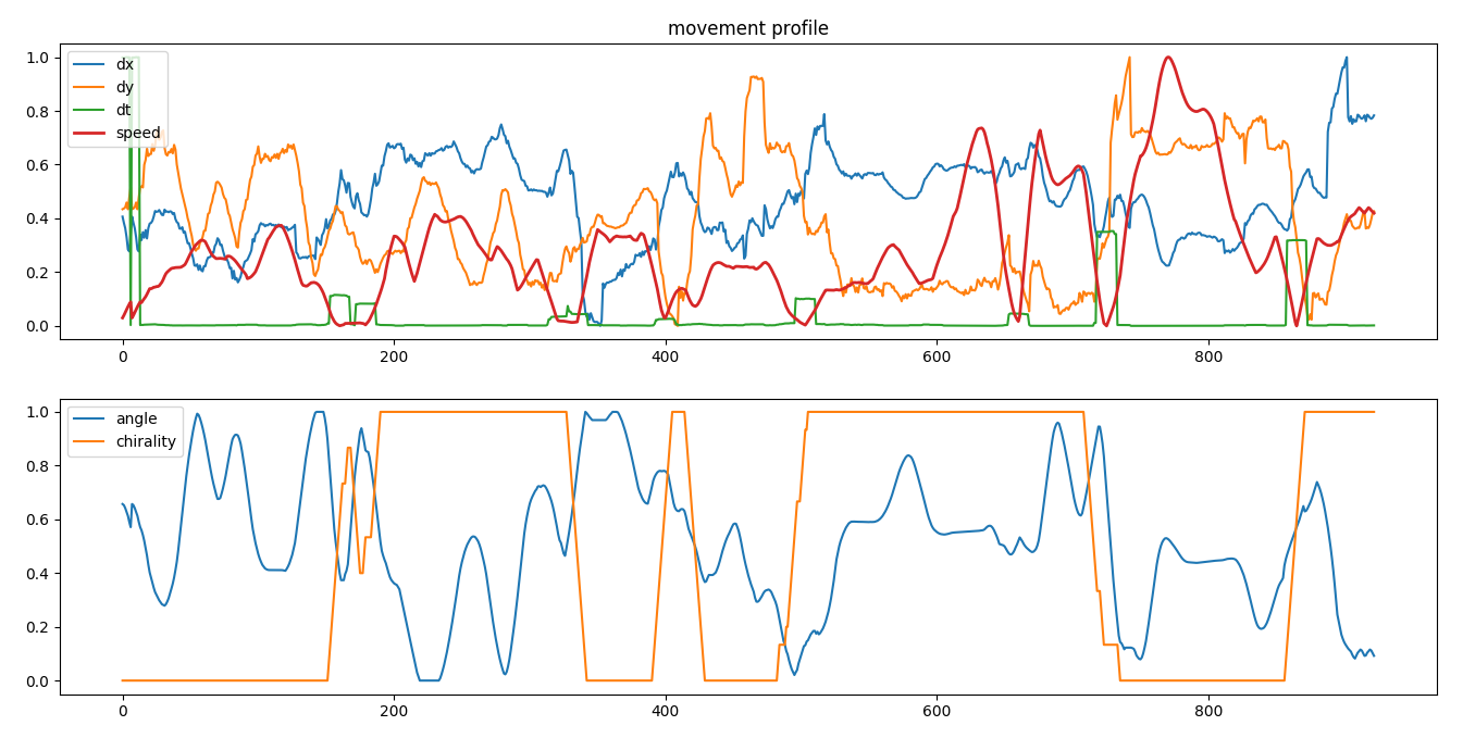 speed,
running average
If we use a Kaiser smoothing we have smooth profiles across all variables.
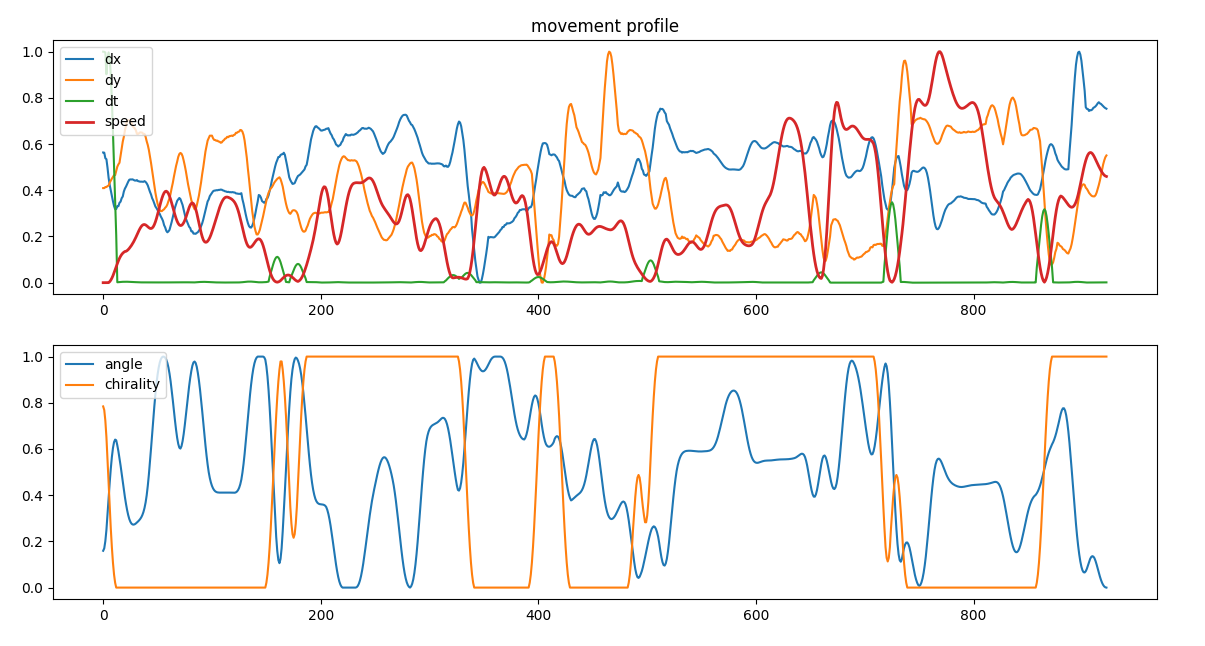 speed, kaiser smoothing
In this way we can calculate the speed density across the city and clearly see the network infrastructure
 speed density
We can also observe the distribution of chirality across the city
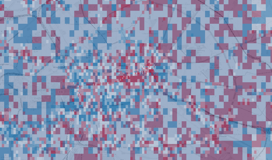 chirality
density
and the distribution of angles, interesting there are some spots strongly polarized
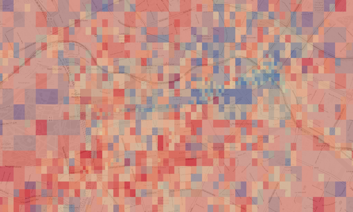 angle density
If we set a speed threshold depending on the particular use case (long/short trips) we can divide motion from dwelling. We cluster the speed profiles when a velocity cross a threshold value. Below the threshold we have a dwelling, above a movement.
mean values
| m_dt | m_x | m_y | m_speed | m_angle | m_chirality | m_m | ||||||
|---|---|---|---|---|---|---|---|---|---|---|---|---|
| 4165 | 13.448 | 52.397 | 1.31E-06 | 1.33 | 0.5 | 1.80E-07 | 1248.57 |
standard deviations
| s_dt | s_x | s_y | s_speed | s_angle | s_chirality | s_m |
|---|---|---|---|---|---|---|
| 0.00026 | 2.58E-05 | 2.62E-06 | 0.553 | 0.234 | 0 |
first and last signal
| x1 | y1 | t1 | x2 | y2 | t2 | sr |
|---|---|---|---|---|---|---|
| 13.44 | 52.3 | 2285.5 | 13.44 | 52.397 | 5196.57 | 0.000143 |
User defined definition of activities and trips
speed profile and the threshold defining
activities
We can display the dwelling and the trips across the city
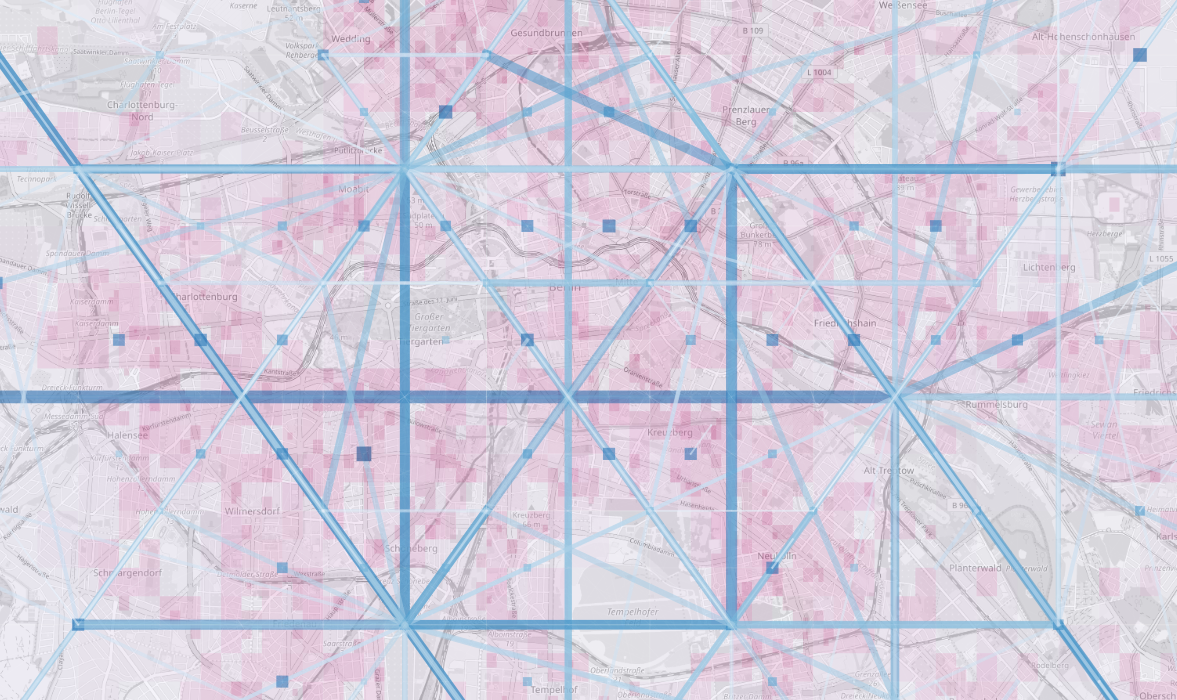 dwelling and moving across the city
Changing the threshold we can distinguish different types of movemens and we have completely different figures
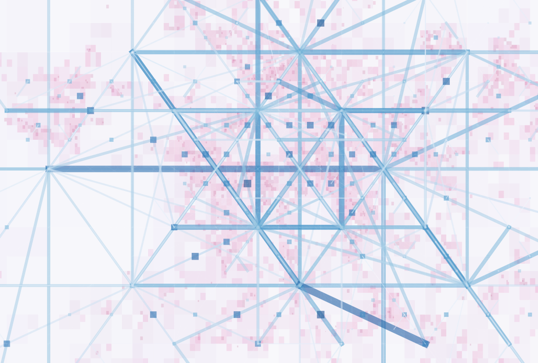 moving and dwelling
We sum up relations grouping first on destinations and than on origins and iterate coarsing the geometry until we reach similar counts per leg.
We have many relations for each node
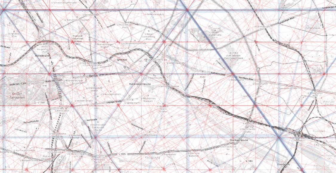 inner city relations
Dwelling can be disconnected from the octree index
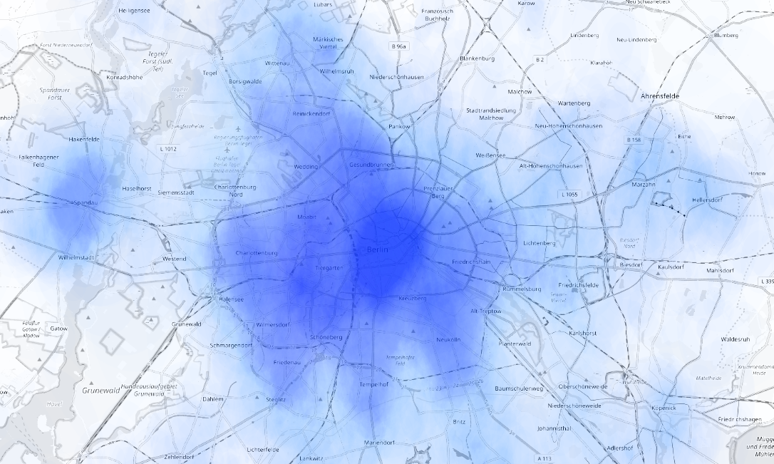 dwelling heatmap
We want to compare mobile antenna connections with gps signal density,
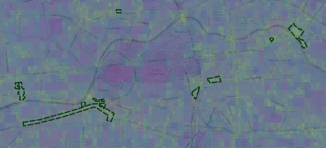 retail areas and densities
Compared to mobile data we have a completely different ranking of locations
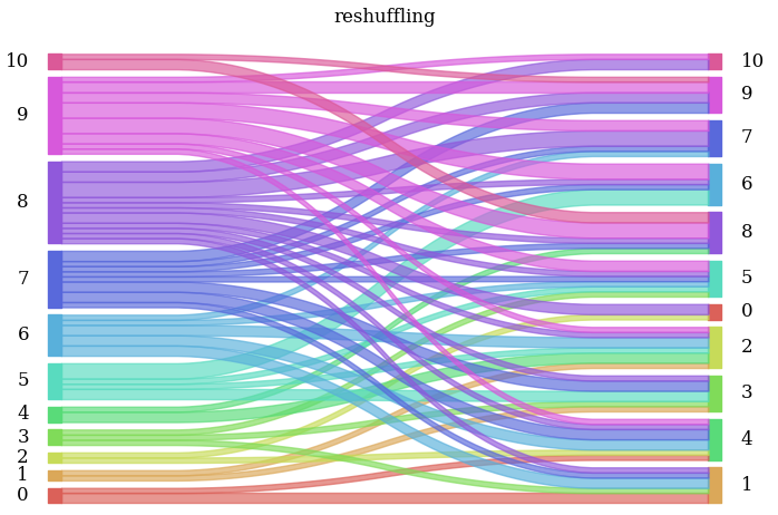 re shuffling of ranking of retail
areas
