Lernia

Lernia is a machine learning library for autmomated learning on geo data and time series.

library description

Content:

• etl
• data cleaning
• feature selection
• feature transformation
• training

modules descriptions

modules are divided into main blocks:

time series

• series_load.py
  • load and preprocess time series mainly from web services
• series_stat.py
  • statistical properties and filtering of time series
• series_forecast.py
  • forecast on time series (arima, holt-winter, bayesian…)
• series_neural.py
  • forecast based on neural networks
• algo_holtwinters.py
  • implementation of holt-winters algorithm

computing

• calc_finiteDiff.py
  • finite difference implementation of differential equations
• kernel_list.py
  • collection of kernels

geographical

• geo_enrich.py
  • enrich location with geographical information
• geo_geohash.py
  • geohash computation
• geo_octree.py
  • octree algebra based on coordinates

basics

• lib_graph.py
  • style for graphs
• proc_lib.py
  • utils for spark processing
• proc_text.py
  • text preprocessing and quantification

learning

• train_reshape.py
  • utils to reshape data prior/post traning
• train_shape.py
  • reduce curves shapes into useful metrics for training
• train_feature.py
  • utils for feature statistics, elimination, importance
• train_interp.py
  • iterpolation for smoothing data
• train_score.py
  • scoring utils for performances
• train_metric.py
  • important metrics for scoring and performance
• train_viz.py
  • visualization utils for performances and data statistics
• train_modelList.py
  • collection of sklearn models to compare performances
• train_model.py
  • iteration and tuning on sklearn models
• train_keras.py
  • parent class for training with keras
• train_deep.py
  • deep learning models for regression and predictions
• train_longShort.py
  • long short term memory models for predicting time sereies
• train_convNet.py
  • convolutional neural networs to predict small images
• train_execute.py
  • execution of learning libraries based on custom problems

Data structure

Every single time series is represented as a

shapeLib

redF = t_s.reduceFeature(X)
redF.interpMissing()
redF.fit(how="poly")
redF.smooth(width=3,steps=7)
dayN = redF.replaceOffChi(sact['id_clust'],threshold=0.03,dayL=sact['day'])
dayN[dayN['count']>30].to_csv(baseDir + "raw/tank/poi_anomaly_"+i+".csv",index=False)
XL[i] = redF.getMatrix()

replace missing

We homogenize the data converting the time series into matrices to make sure we have data for each our of the day. We than replace the missing values interpolating:

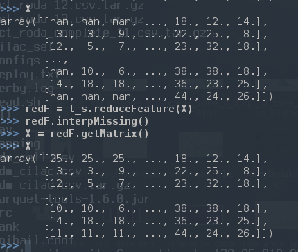replace missing values via interpolation

smoothing

In order to compensate the effects of time shifting (can counts double within two hours?) we apply a interpolation and smoothing on time series:

to the raw reference data we apply: 1) polynomial interpolation 2) smoothing

chi square distribution

Some locations are particularly volatile and to monitor the fluctuations we calculate the χ² and control that the p-value is compatible with the complete time series. We substitute the outliers with an average day for that location and we list the problematic locations.

Distribution of p-value from χ² for the reference data

We than replace the outliers:

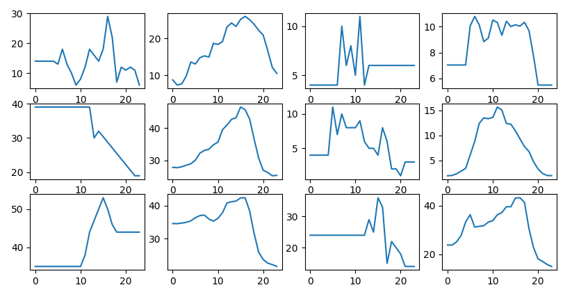outliers are replaced with the location mean day, left to right

feature importance

We studied the statistical properties of a time series collecting the most important features to determine data quality. 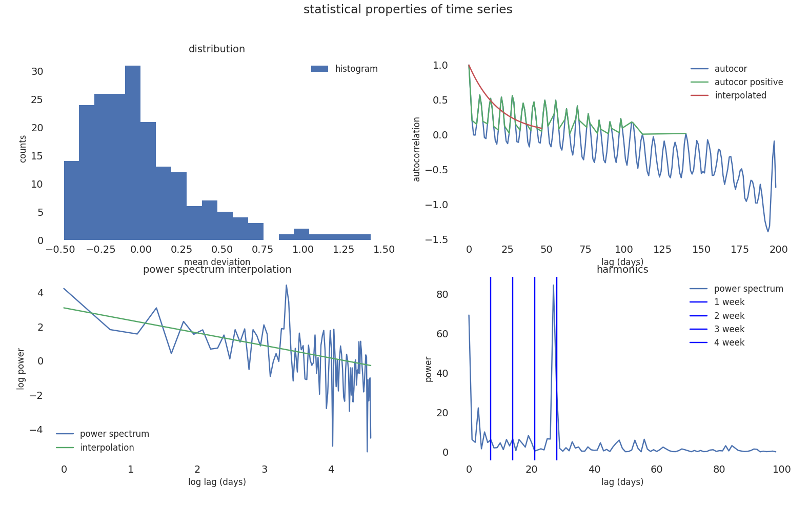most important statistical properties of time series

We calculate the feature importance on model performances based on statistical properties of time series of reference data. 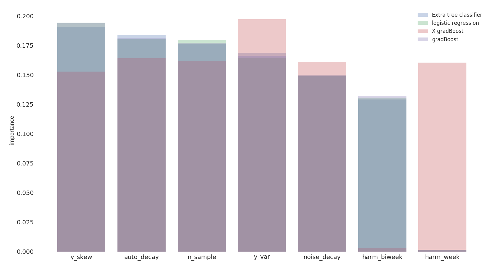we obtain a feature importance ranking based on 4 different classification models

• daily_vis: daily visitors
• auto_decay: exponential decay for autocorrelation –> wie ähnlich sind die Tagen
• noise_decay: exponential decay for the power spectrum –> color of the noise
• harm_week: harmonic of the week –> weekly recurrence
• harm_biweek: harmonic on 14 days –> biweekly recurrence
• y_var: second moment of the distribution
• y_skew: third moment of the distribution –> stationary proof
• chi2: chi square
• n_sample: degrees of freedom

We try to predict model performances based on statistical properties of input data but the accuracy is low which means, as expected, that the quality of input data is not sufficient to explain the inefficiency in the prediction. 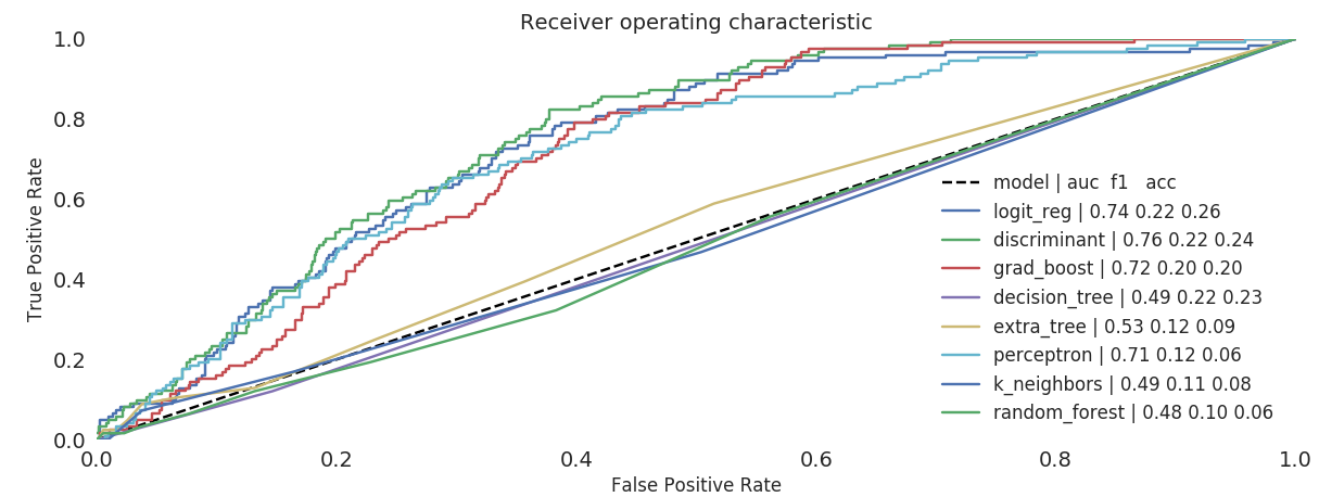training on statistical properties of input data vs model performances

We now extend our prediction based on pure reference data and location information 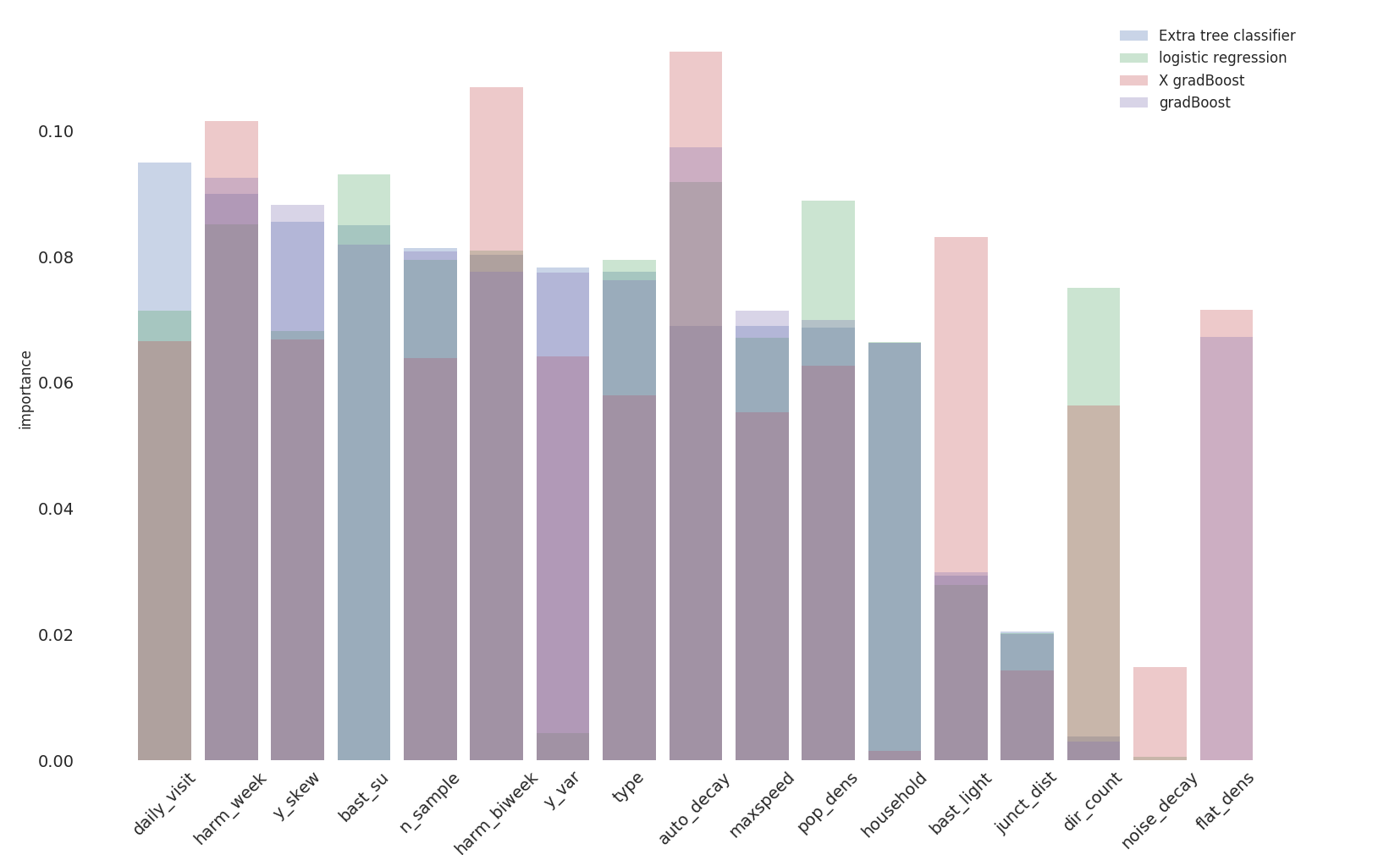feature importance based on location information and input data

Knowing the location information we can predict the performace within 80% of the cases. 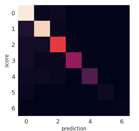confusion matrix on performance prediction based on location information

reduce features

We select the most relevant weather features over a selection of 40. 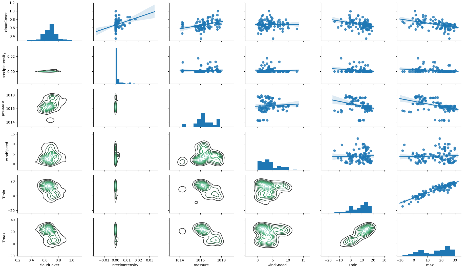correlation between weather features

Other weather related parameters have an influence on the mismatch. 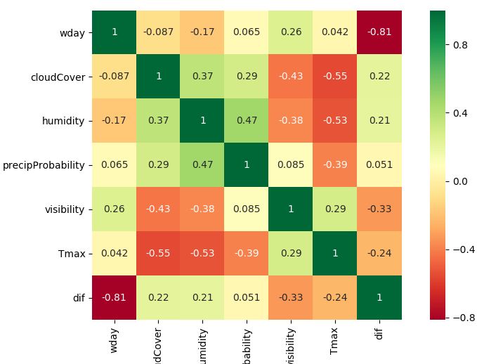weather has an influence on the deviation: di../f/f

We use the enriched data to t

Regression

All the skews we have shown are used to train predictors and regressors to adjust counts: 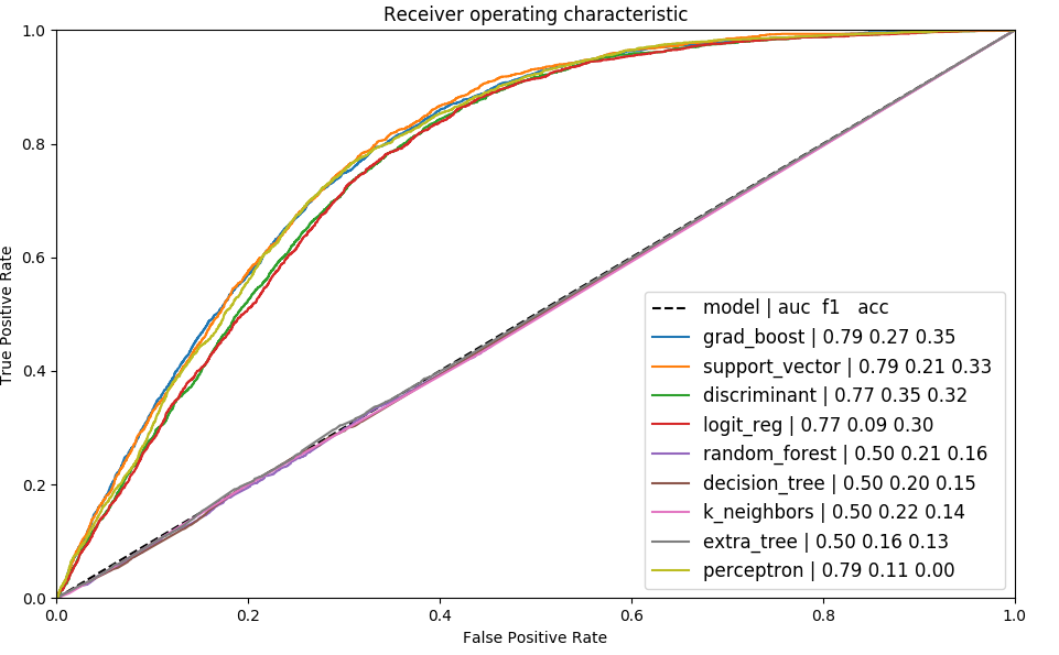ROC of different models on training data

Thanks to the different corrections we can adjust our counts to get closer to reference data. 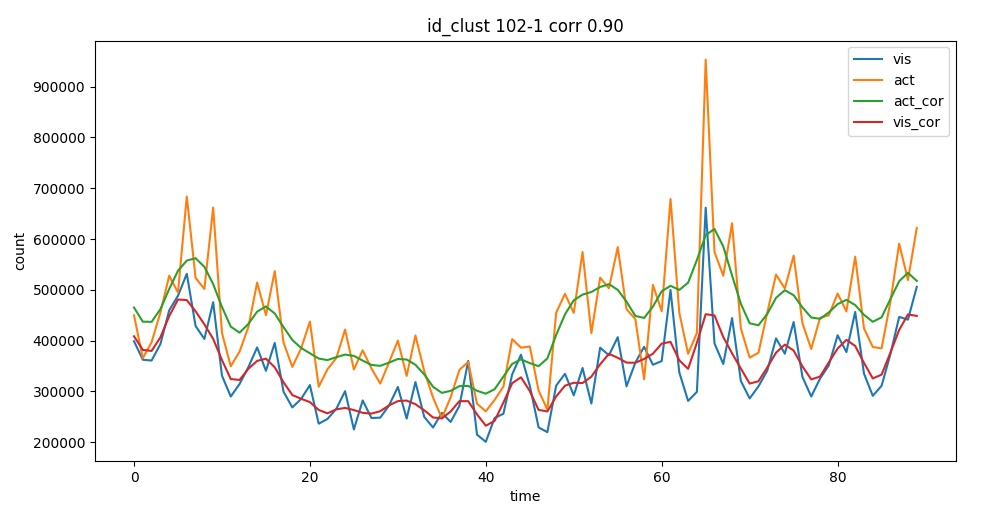corrected activities after regressor

We have structure the analysis in the following way: 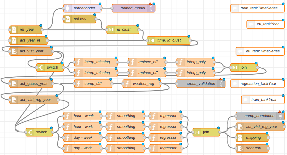structure of the calculation for the yearly delivery

We can than adjust most of the counts to meet the project KPIs

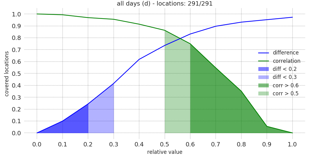distribution of the KPIs ρ and δ

Shape clustering

We want to recognize the type of user clustering different patterns:

different patterns for kind of user

We calculate characteristic features by interpolating the time series. We distinguish between a continous time series where we can calculate the overall trends via the class train_shapeLib.py

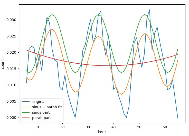time series of a location and the daily average where we can understand the typical daily activity.

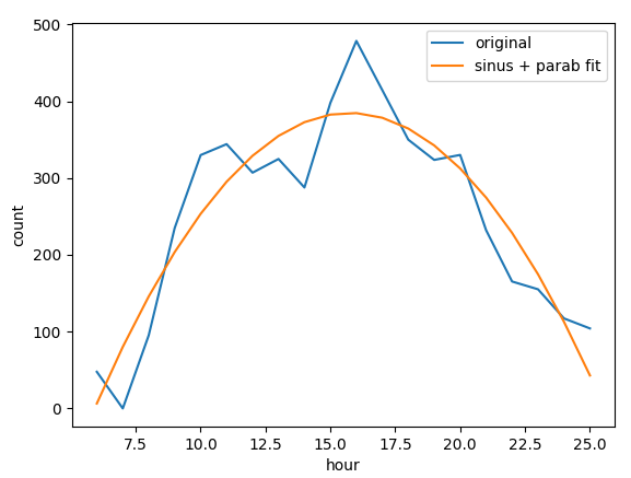daily average of a location Many different parameters are useful to improve the match between mobile and customer data, parameters as position of the peak, convexity of the curve, multiday trends help to understand which cells and filters are capturing the activity of motorway stoppers.

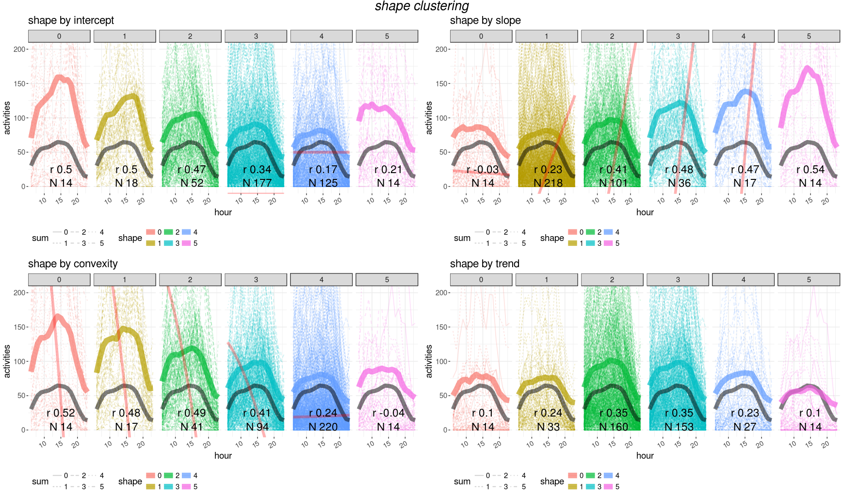clustering curves (average per cluster is the thicker line) depending on different values of: intercept, slope, convexity and trend

Unfortunately no trivial combination of parametes can provide a single filter for a good matching with customer data. We need then to train a model to find the best parameter set for cells and filter selection.

Feature selection

We need to find a minimal parameter set for good model performances and spot a subset of features to use for the training. We realize that some features are strongly correlated and we remove highly correlated features

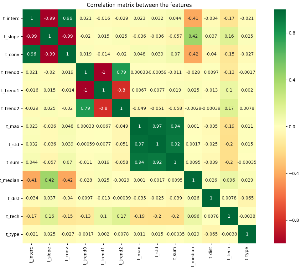correlation between features

High variance can signify a good distribution across score or a too volatile variable to learn from.

We select five features which have larger variance to increase training cases.

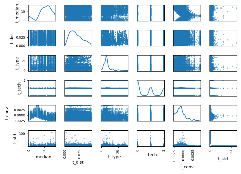final selection of features

Scoring

We use the class train_shapeLib.py to calculate the score between users data and customer data. We calculate the first score, _cor, as the Pearson’s r correlation: $$ r = \frac{cov(X,Y)}{\sigma_x \sigma_y} $$ This parameter helps us to select the curves which will sum up closely to the reference curve.

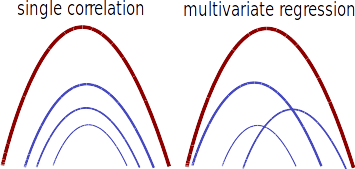the superposition of many curves with similar correlation or many curves with heigh regression weights leads to a good agreeement with the reference curve The second parameter, the regression _reg, is the weight, w, given by a ridge regression $$ \underset{w}{min\,} {{|| X w - y||_2}^2 + \alpha {||w||_2}^2} $$ where α is the complexity parameter.

The third and last score is the absolute difference, _abs, between the total sum of cells and reference data: $$ \frac{|\Sigma_c - \Sigma_r|}{\Sigma_r} $$ per location

libKeras

deep learning autoencoder

We build an autoencoder which is a model that learns how to create an encoding from a set of training images. In this way we can calculate the deviation of a single image (hourly values in a week 7x24 pixels) to the prediction of the model.

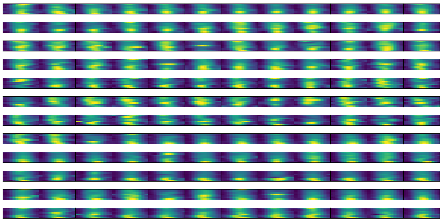sample set of training images, hourly counts per week

In this way we can list the problematic locations and use the same model to morph measured data into reference data.

We train a deep learning model on images with convolution: 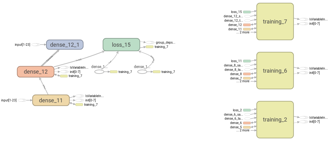sketch of the phases of learning

We than test how the images turn into themselves after the prediction of the autoencoder.

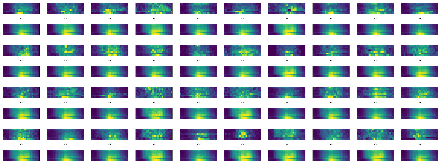comparison between input and predicted images

We can than state that 88% of locations are not well predictable by the model within 0.6 correlation. 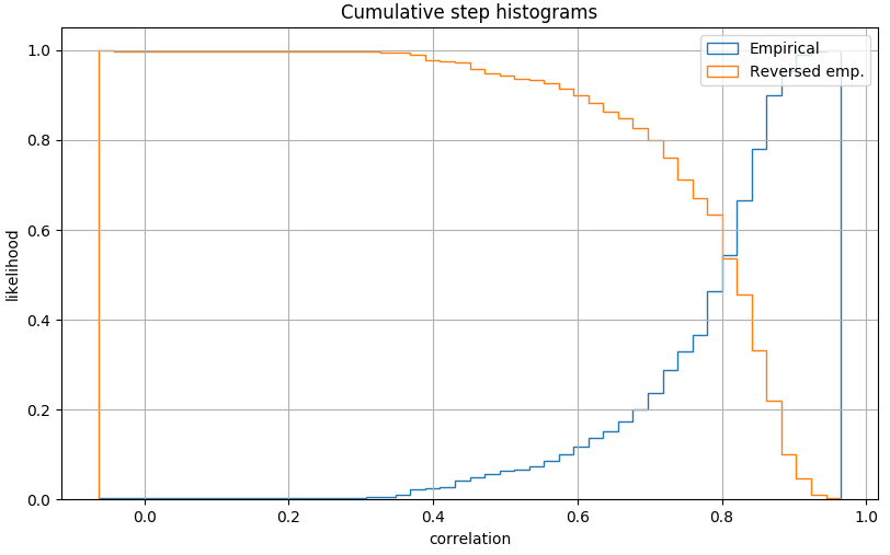distribution of correlation for autoencoder performances: correlation on daily values

implementation

Results generation

Applying both predictor and regressor and we generate: 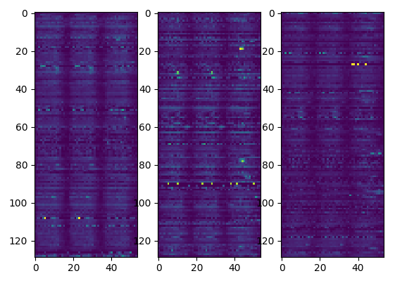resulting activities per location

We then sort the results depending on a χ² probability and discard results with an high p_value 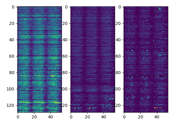activities sorted by p-value

To summarize we generate the results applying the following scheme: 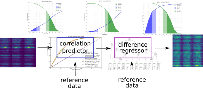application of the predictor and regressor

The detailed structure of the files and scripts is summarized in this node-red flow charts: 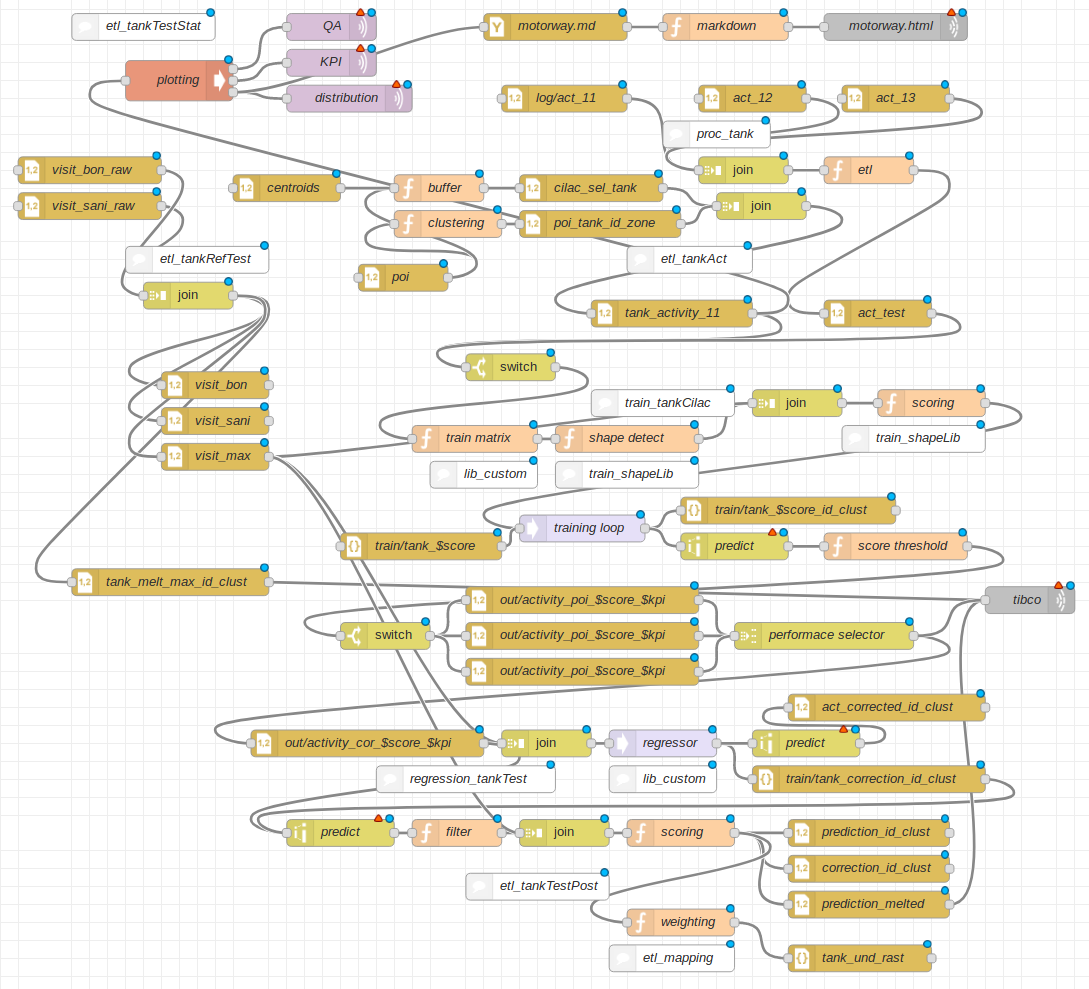flow chart of the project

We have structure the analysis in the following way: structure of the calculation for the yearly delivery