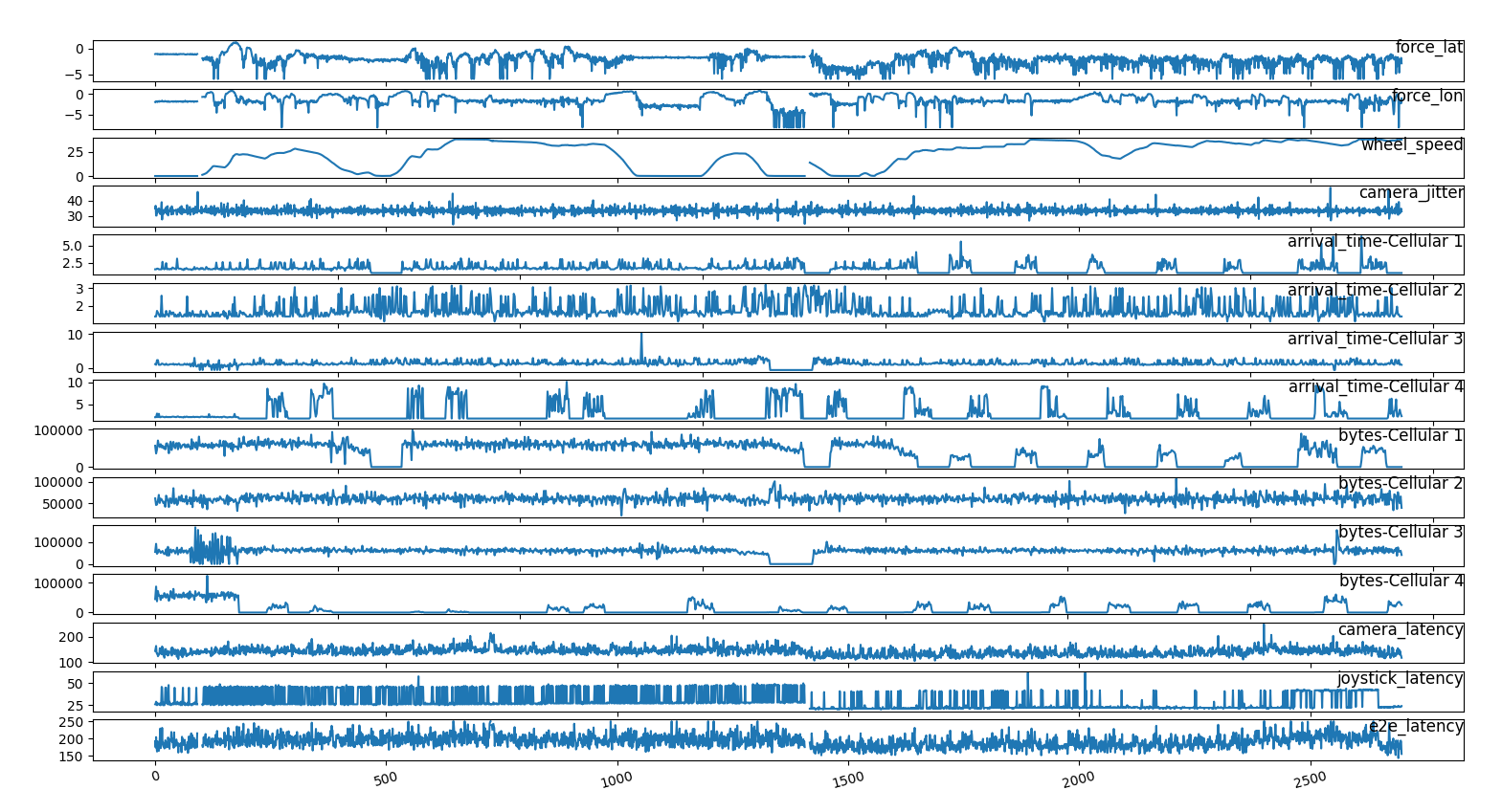
 time series of the most relevant
features
time series of the most relevant
featuresDefinition and prepartation of the data sets
Source: etl_telemetry_deci Query: network_log.sql
To analyze the deci second data we can use fewer features (because of
sampling rate) like the computing features and
vehicle_ping. Event rtp and modem
features have to be removed. We collect other networking
features from the network_log table where we subset the
telemetry data into a series of spikes and we merge the network data
information using the timestamp and the
vehicle_id. We pivot the network_log table wrt
to the modem name. We also discard ttl and
interval_duration for the low information contained. We
discard packets because the hava a correlation of 0.98 with
bytes.
 time series of the most relevant
features
We see that the quantity of transmitted information slightly correlates between modems signalizing similar networking issues across operators. The correlation between bytes and arrival time is lower than expected
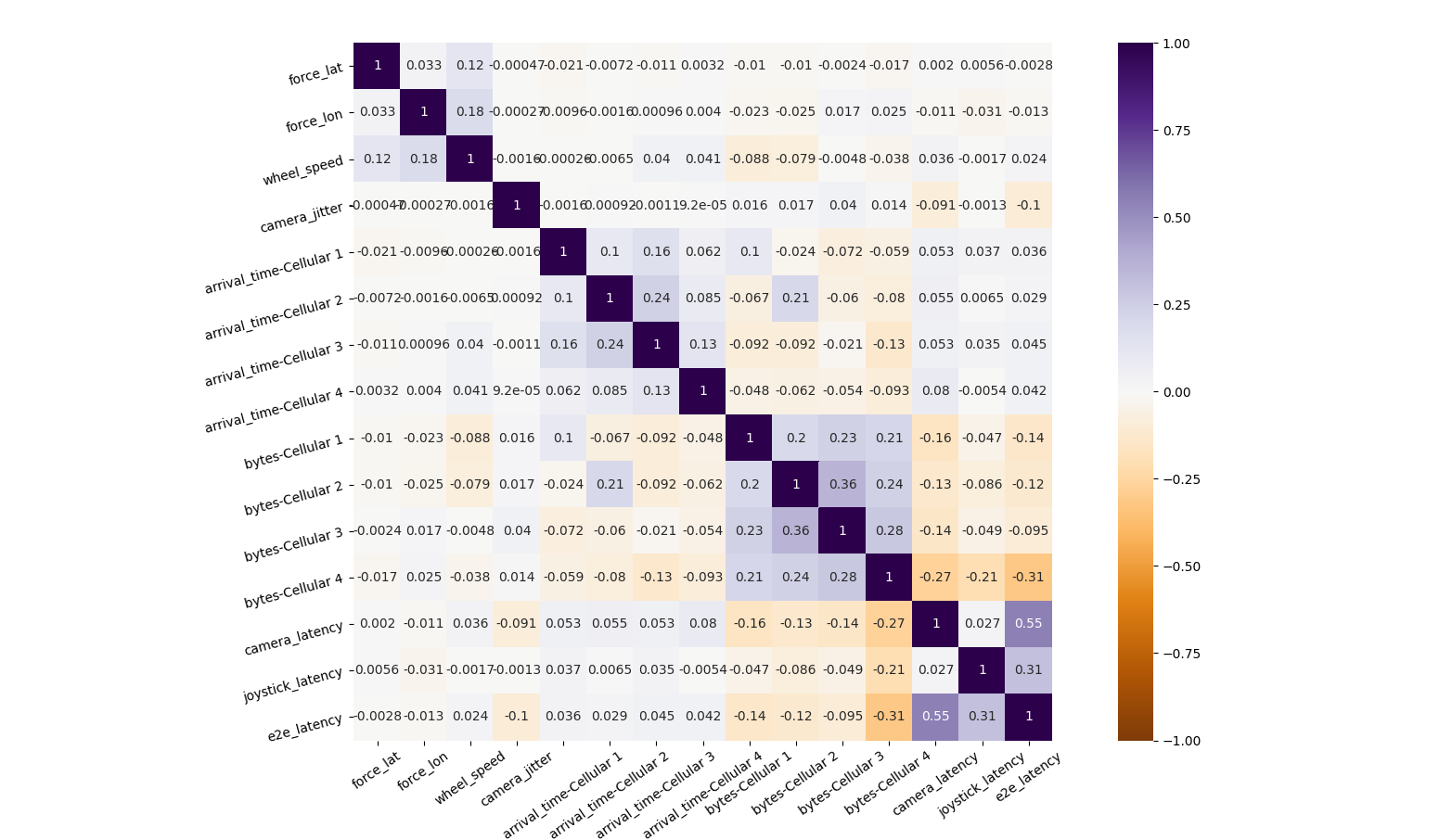 correlation between the network log features
But in general modems have a different behaviors, cellular 3 is the most stable and transmits more data.
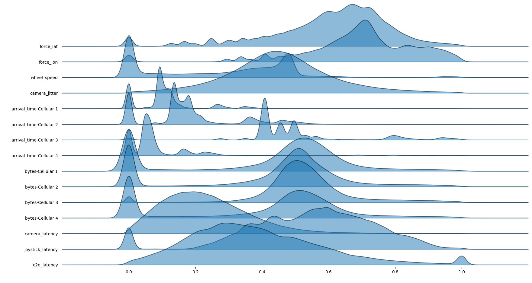 joyplot of network_log
features
We prepare different datasets for different parts of the analysis:
The different sets have a different sampling of events, the
latency set has few spike events while the
spike set has all the perturbations before and after a
disruption event.
From the two dataset we can see the different feature distribution and feature importance.
Query: resample_1sec Code: etl_spikes
We resample averaging 1 sec worth of data but some fields are still uncomplete, around 1% of the timse
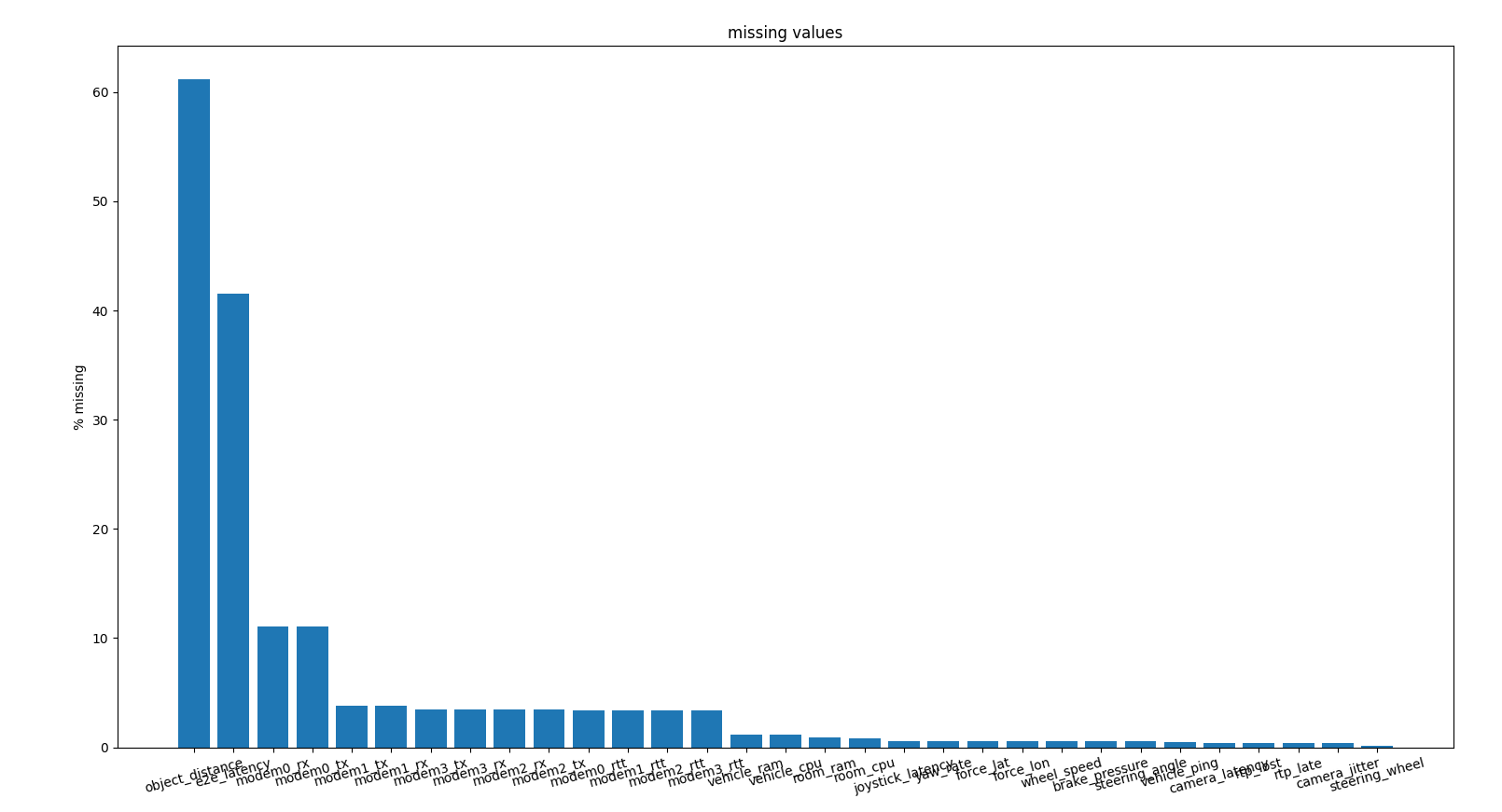 percentage of missing data in certain features
We identify the peak and split each time series in sub series where all peaks are aligned at the minute 4 and we leave one minute after the spike.
We artificially exagerate the peak to help the model understand it and set the peak max value to a plateau
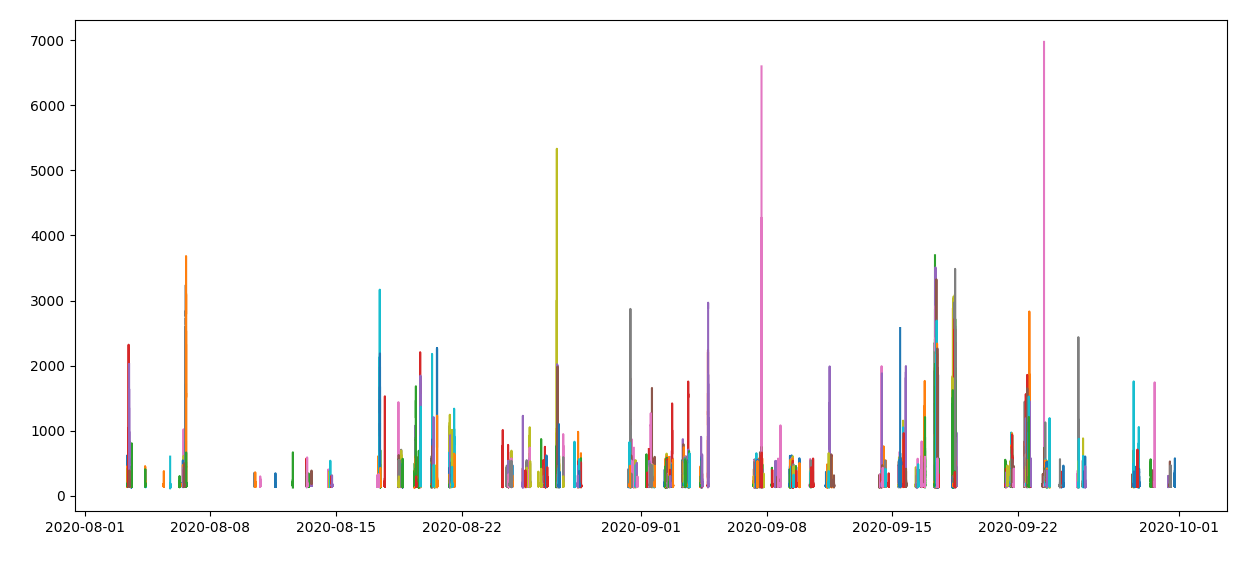 series of spikes
We than abstract the time and create a stack of series where the peak in phase
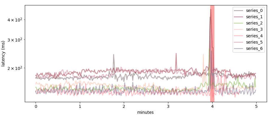 stack
of spikes where the spike happens at minute 4
It is interesting to analyze some spike series to understand qualitatively what might happen during incidents. In this case we see two concurrent spikes in two different sessions
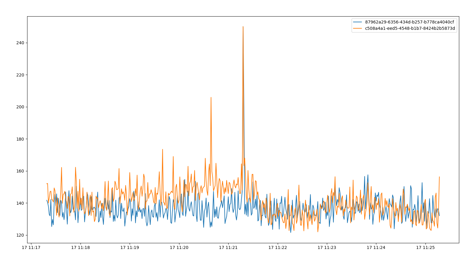 two spikes at the same time on different
cars (24, 76)
Averaging the two series it seems that the room_cpu has
a clear variation prior to the spike.
 average of both time series prior to
the spike
We see 3 of such pairs: 2020-08-17T11, 2020-08-24T18, 2020-08-20T08.
At first we discard poor features analyzing:
Spikes are rare events and some features might be as rare as spikes
and than a indication of them but in case of
['td_brake','td_throttle','steering_interval'] we see that
data are rare don’t happen in high latency cases.
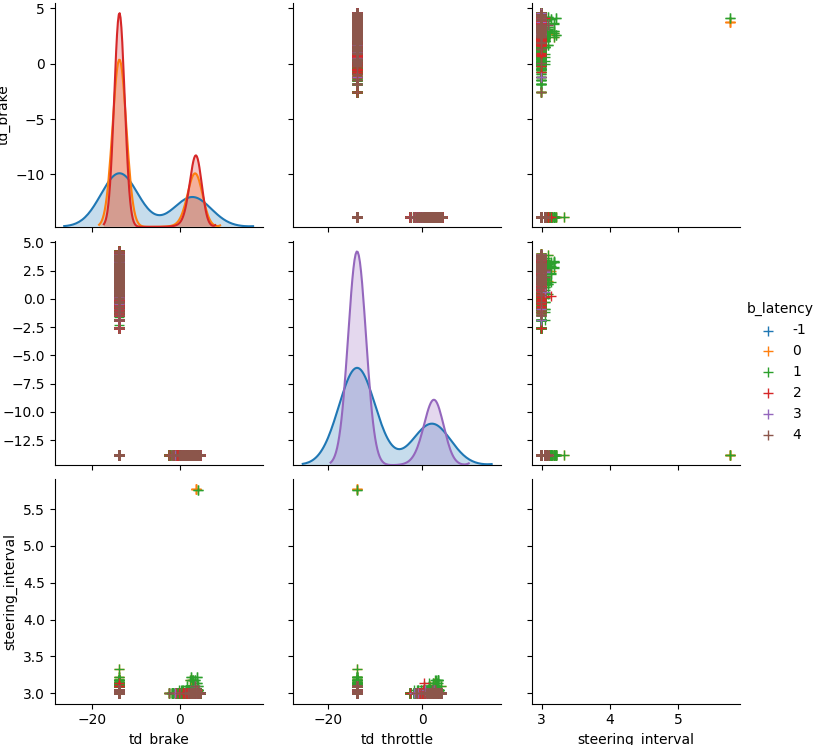 poor features
In comparison we see that rtp_lost and
rtp_late have a clear distribution dinstinction although
most of the time data are NaNs
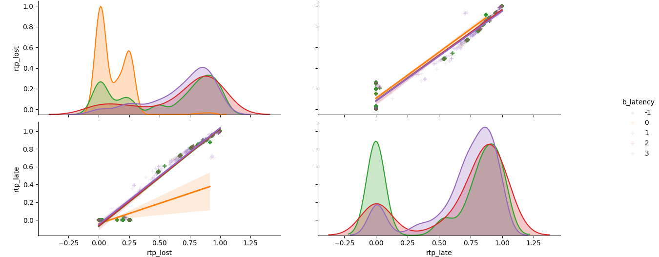 poor features but discriminators for latency
Code: stat_telemetry, stat_latency.
Of the most important feature we visualize the time series
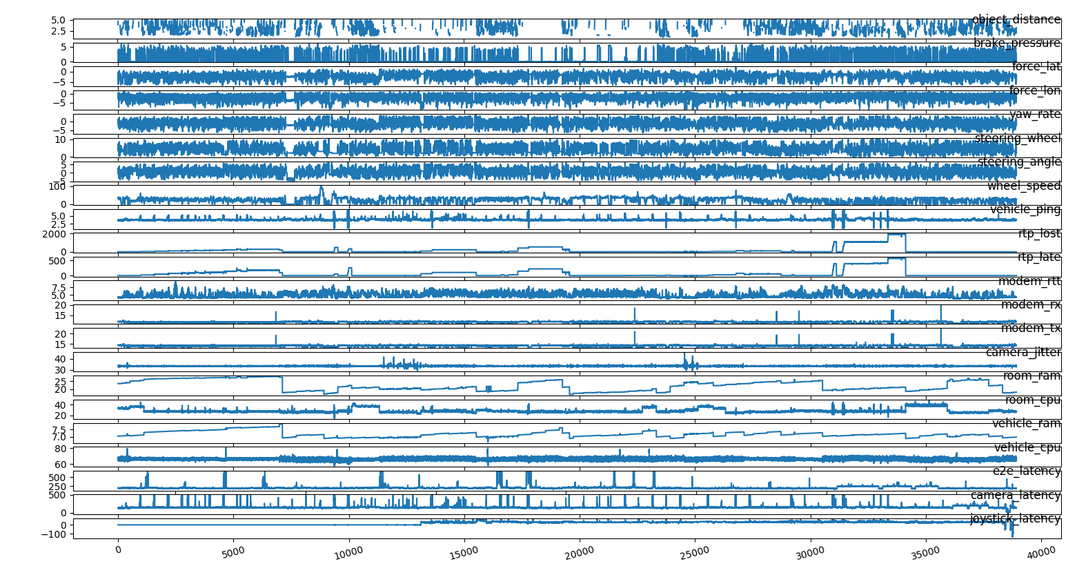 visualization of the time series
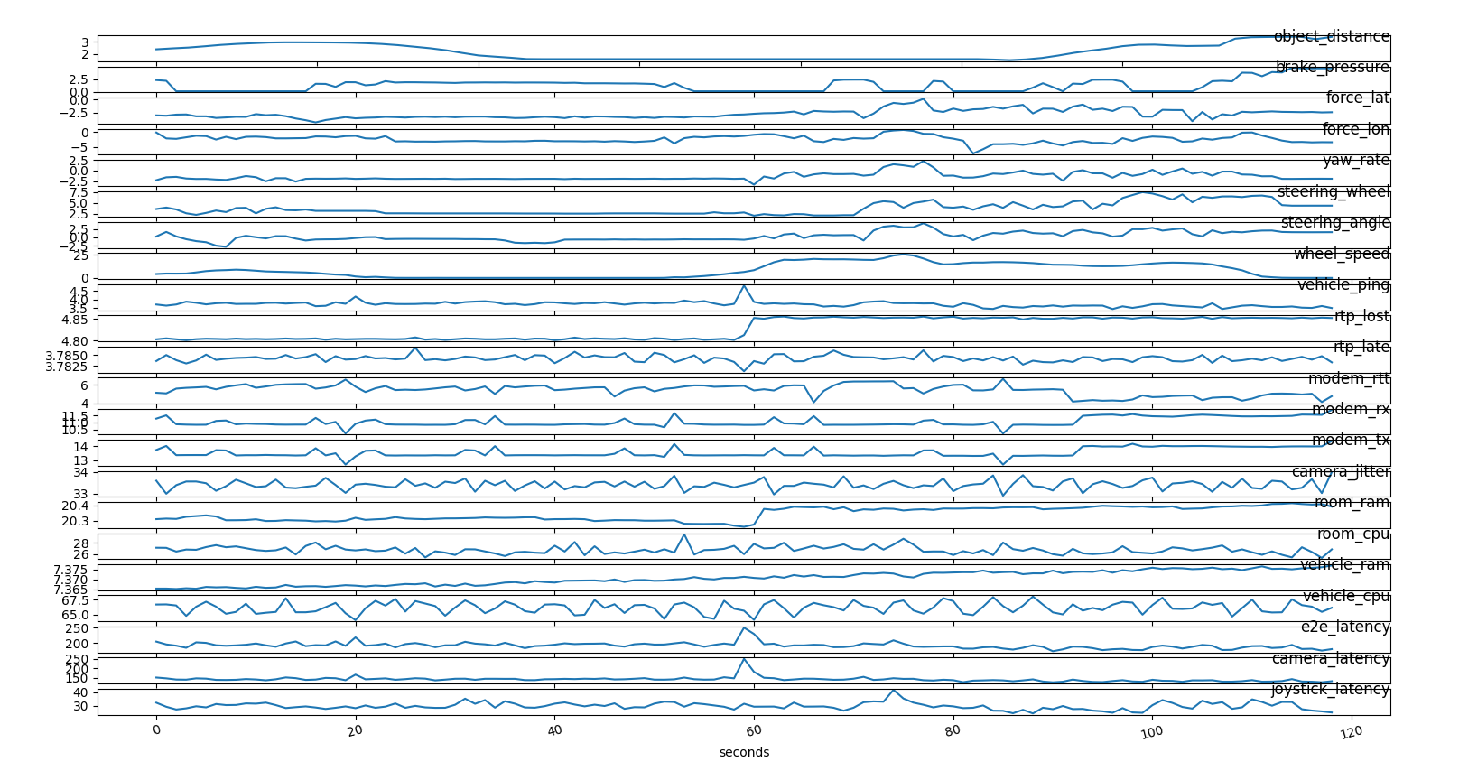
We collect a day of data and subset the time series prior to a spike
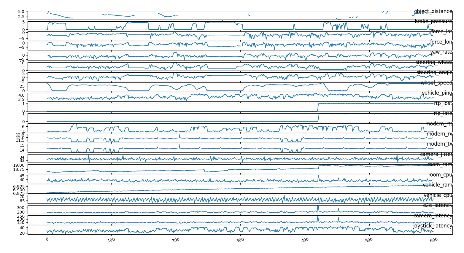 time series of the most relevant features prior
to a spike, we can see that after the disruption the vehicle
brakes
We removed some features because of the obvious cross correlation
(ex: brake_pressure ~ wheel_speed)
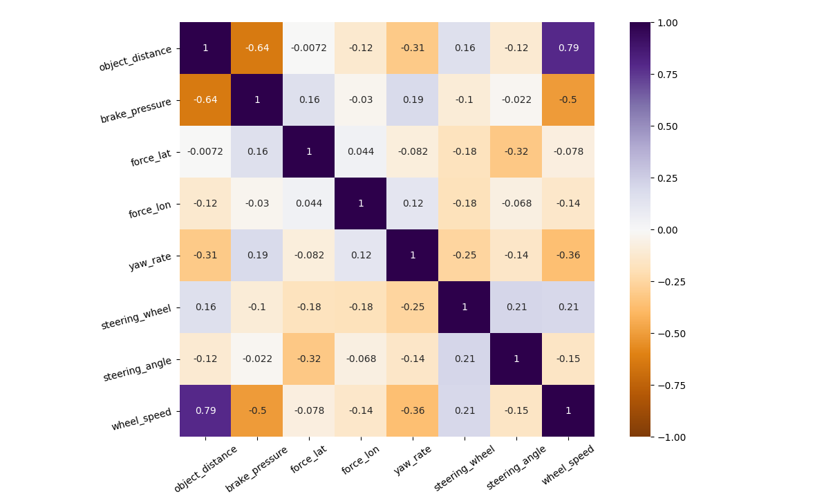 feature
correlation, obvious cross correlation
We see a dependency between vehicle and
control_room cpu and ram
usage
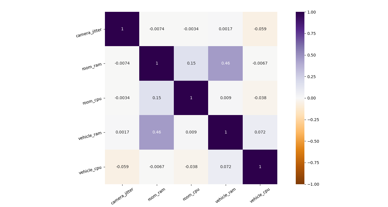 vehicle and control room interdependency on
computation
We see that not all the features are distributed regularly and some are pretty noisy.
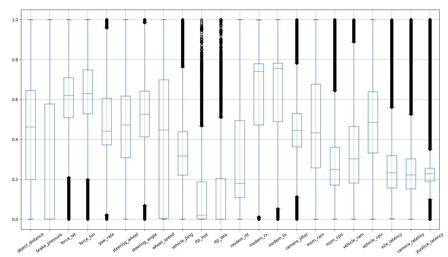 distribution of the latency features:
boxplots
In case of the spike subset the distribution get a bit broader
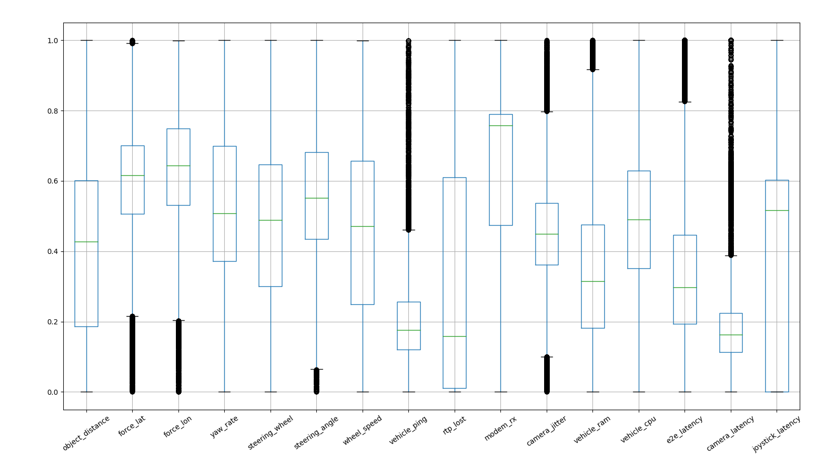 distribution of the spike features:
boxplots
We than calculate the logaritmic of the most dispersed features
(e.g. _force_) to gain more meaningful information.
Changing the latencies to their logaritmic value doesn’t change much the
distributions
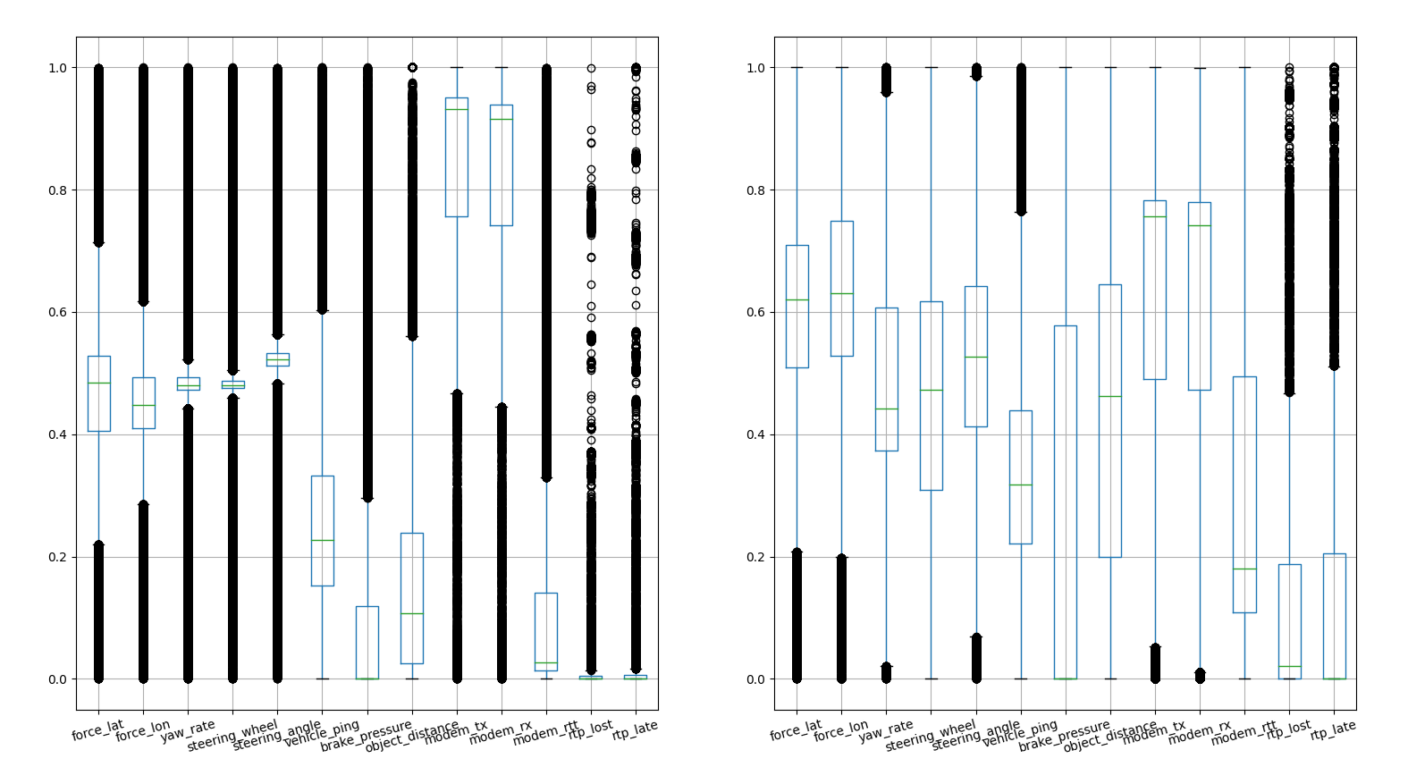 logaritmic transformation for some
features
We see that some quantities are bimodal, interestingly latencies too. It seems there are clear distinguished operating regimes.
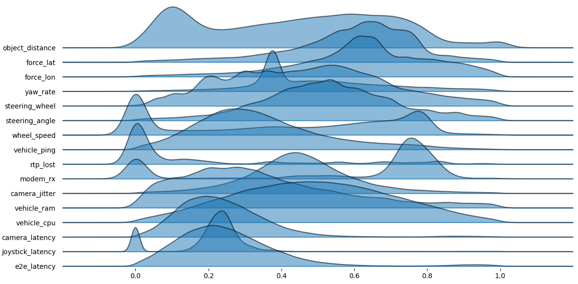 distribution of the latency features:
joyplots
Another feature selection takes more into account the networking features, the different time frames change a lot the data distribution. In this case we consider only events in the proximity of a spike and the features become even more bimodal
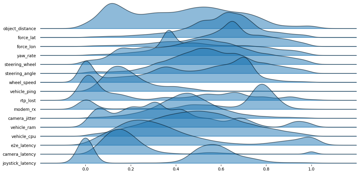 distribution of the spike features:
joyplots
Looking at the pair plot we see that only ram_usage has
an interesting dependency on the camera_latency, the
**purple set is the one corresponding to the larger bin of the
camera_latency
We analyze the how the networing features distributes in different regimes of camera latency
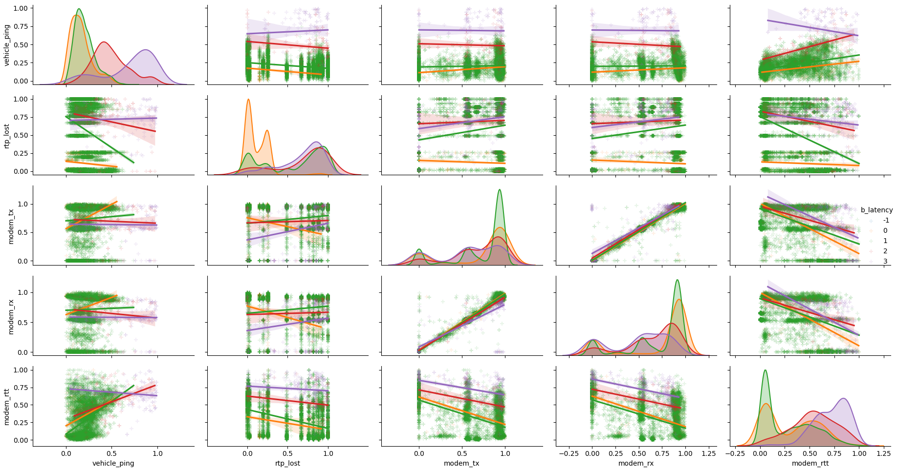 pairplot of the networking features
Same for the computing features
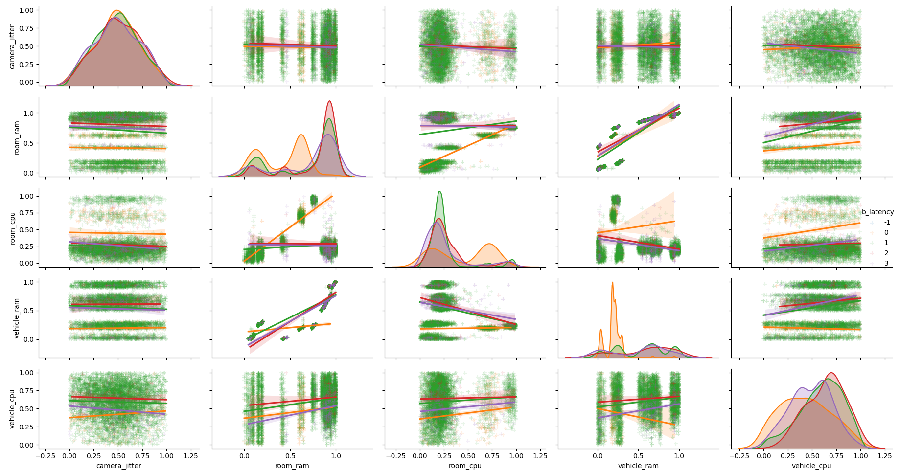 pairplot of the computing features
Pairplot for vehicle dynamics features don’t show a clear dependency on latency
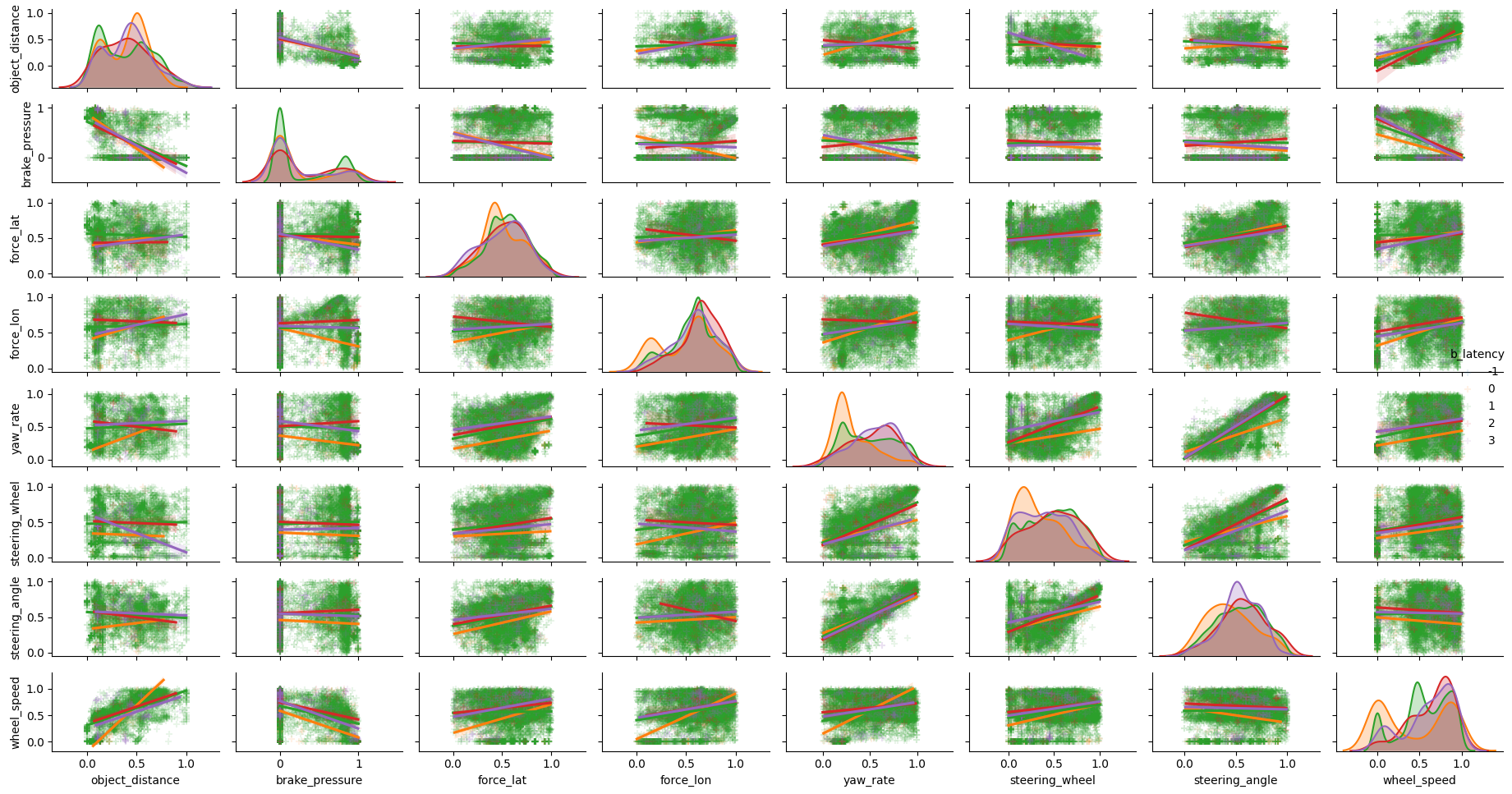 pairplot of the vehicle dynamics features
We want to understand the periodicity and auto correlation of
camera_latency to understand how to separate different
regimes
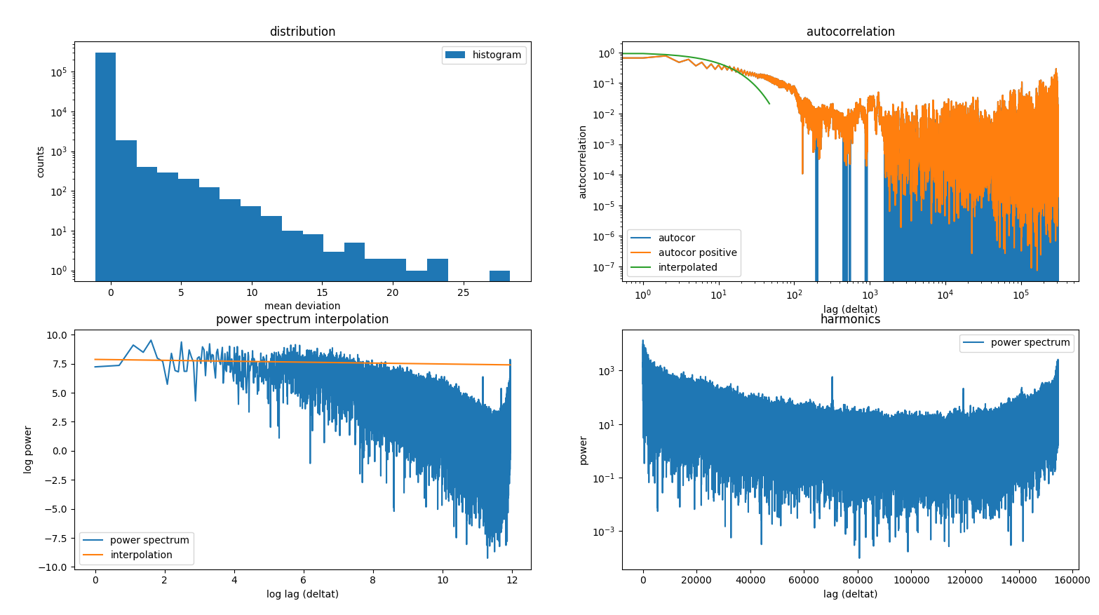 latency decays and frequency behaviour
We analyze the power spectrum for a normal latency or during a spike
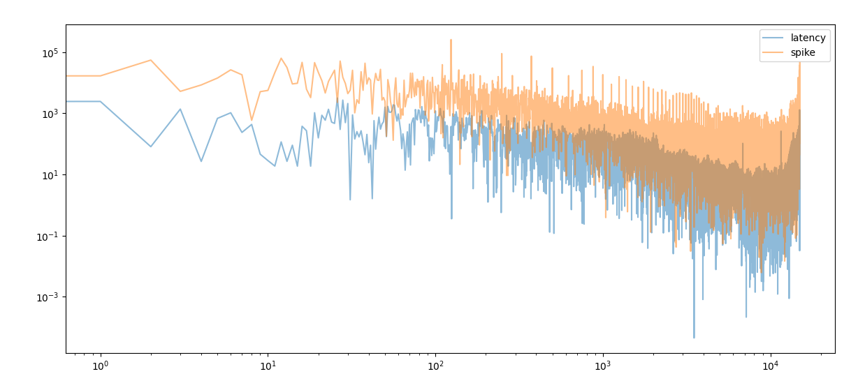 latency power spectrum for normal and spike regimes
During the spike event autocorrelation is a bit larger and more stable than in the normal regime
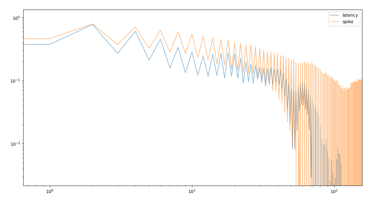 Autocorrelation for camera latency in normal and spike
regimes
For a fast and reliable training a good normalization is essential for the performances of the predictions. We need to find a stable normalization to keep across all predictions. If we need to change the normalization than we need to retrain the model.
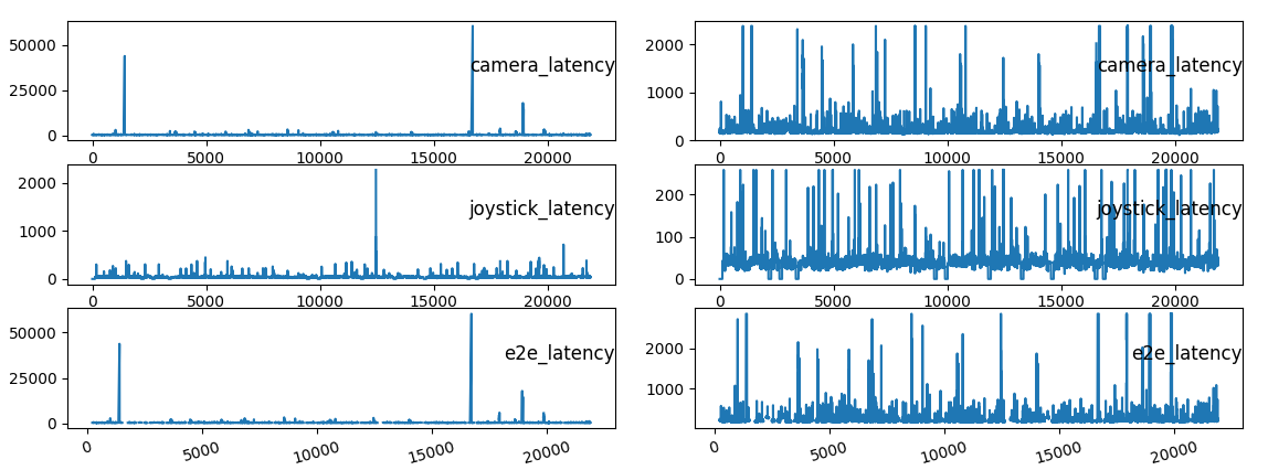 flattening of outlier to let the normalization to operate in a
consitently populated regime
To have a clear understanding on what is happening we stack many time series where the spike happens at the 0 second. We take 160+ time series and we calculate the average to denoise and have a more statistical understanding on the process
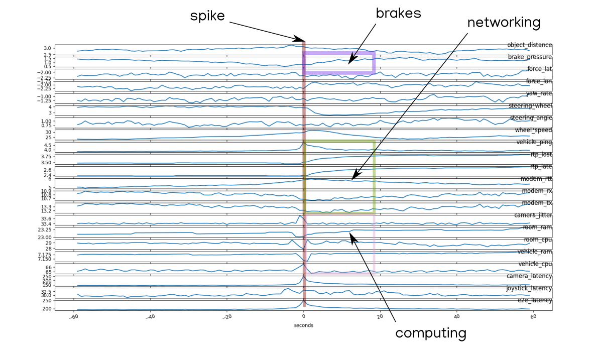 average on spike events where the spike happens at second 0
If we have a clear look at the moment where the spike happens we clearly see that some features show a change previous to the spike and others consequent to the spike
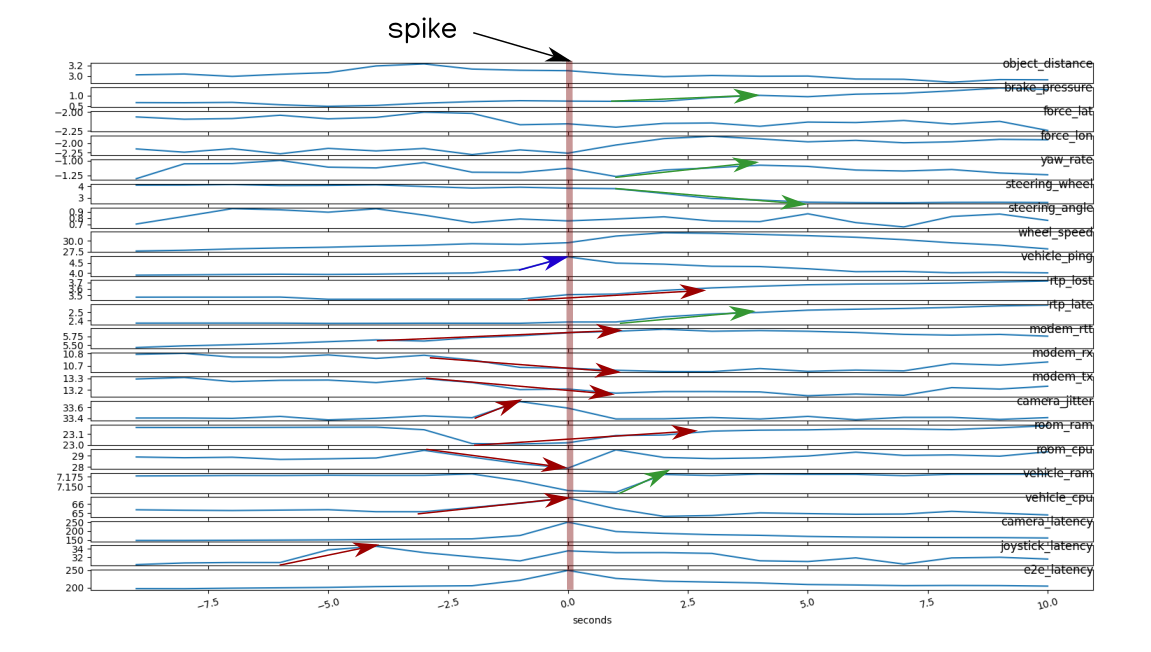 detail on the few seconds around the spike
event
Similarly we look at the signal differences
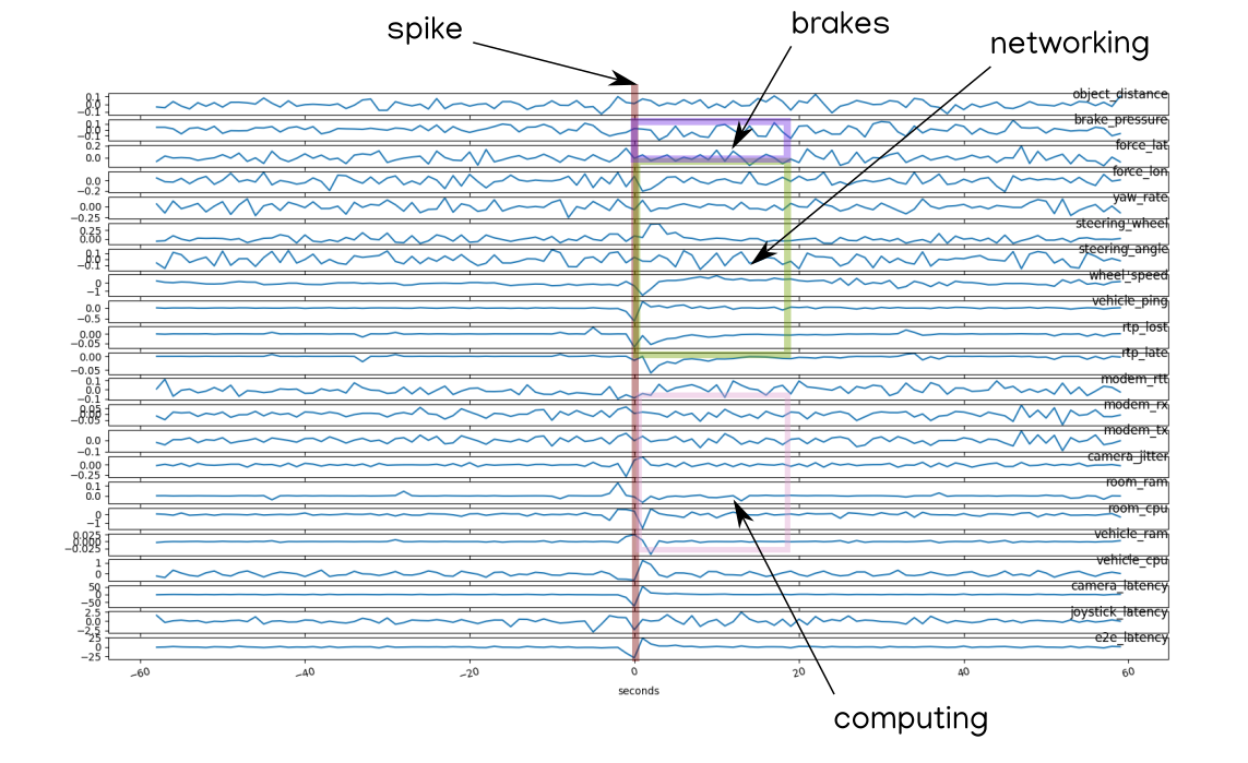 series evolution of the feature differences
and the close up
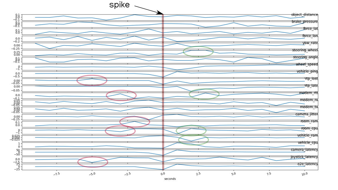 series evolution of the feature
differences
We analyze the variance depending on the time to the spike
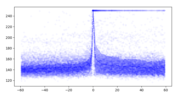 variance of camera latency
Another important indicator of causal dependency is the dropping of
variance before a spike which tell us that
ram is clearly affected by spikes
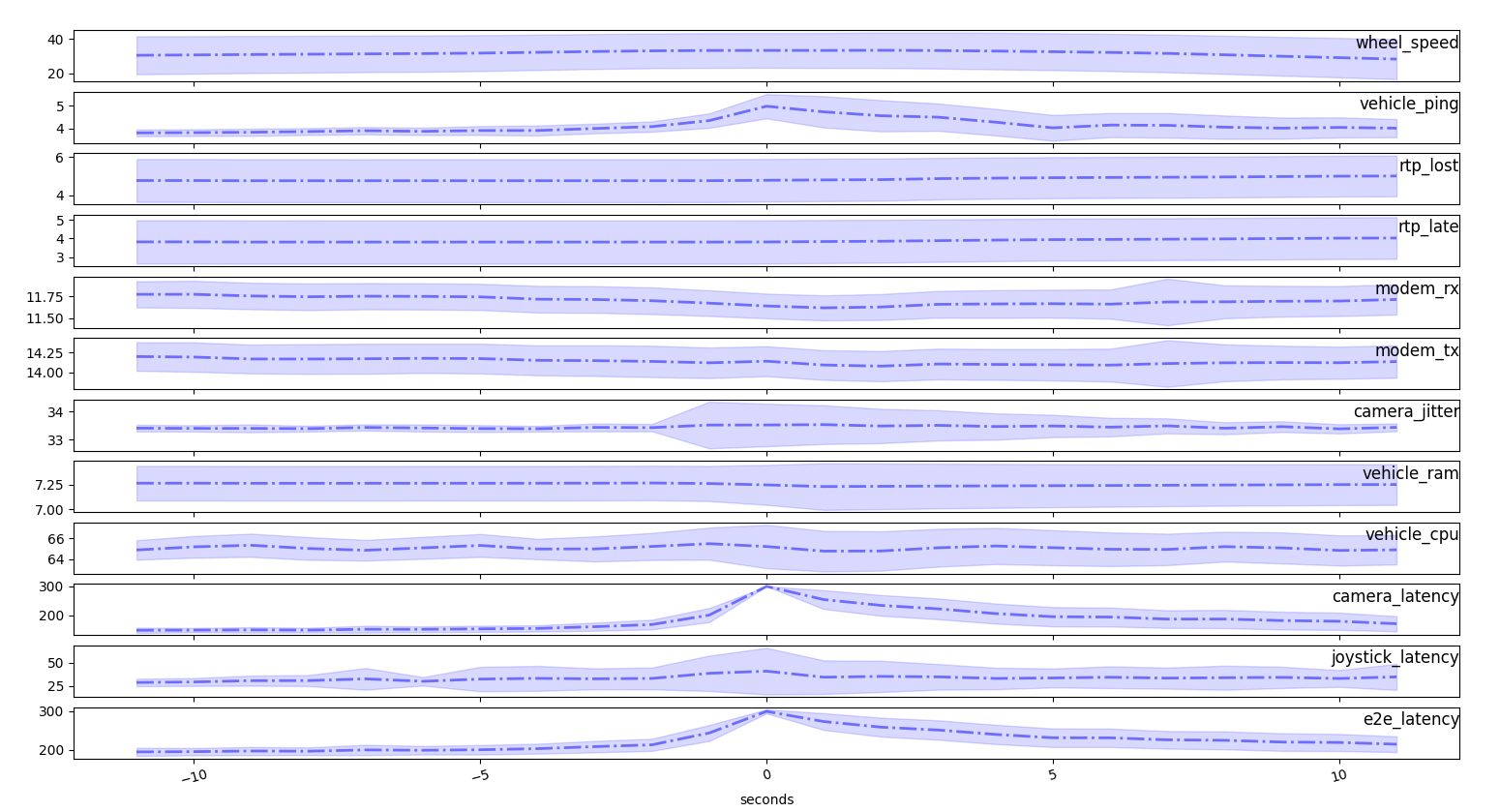 variance of time series
For some features the variance is so high that we would consider the averages just random fluctuations
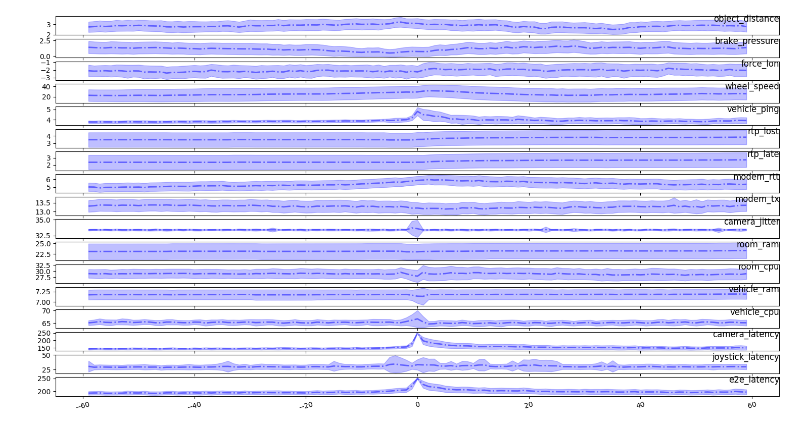 variance and mean for time series
We analyze the time series for the features with an higher firing rate, we see that in average the byte volume drops across all modems
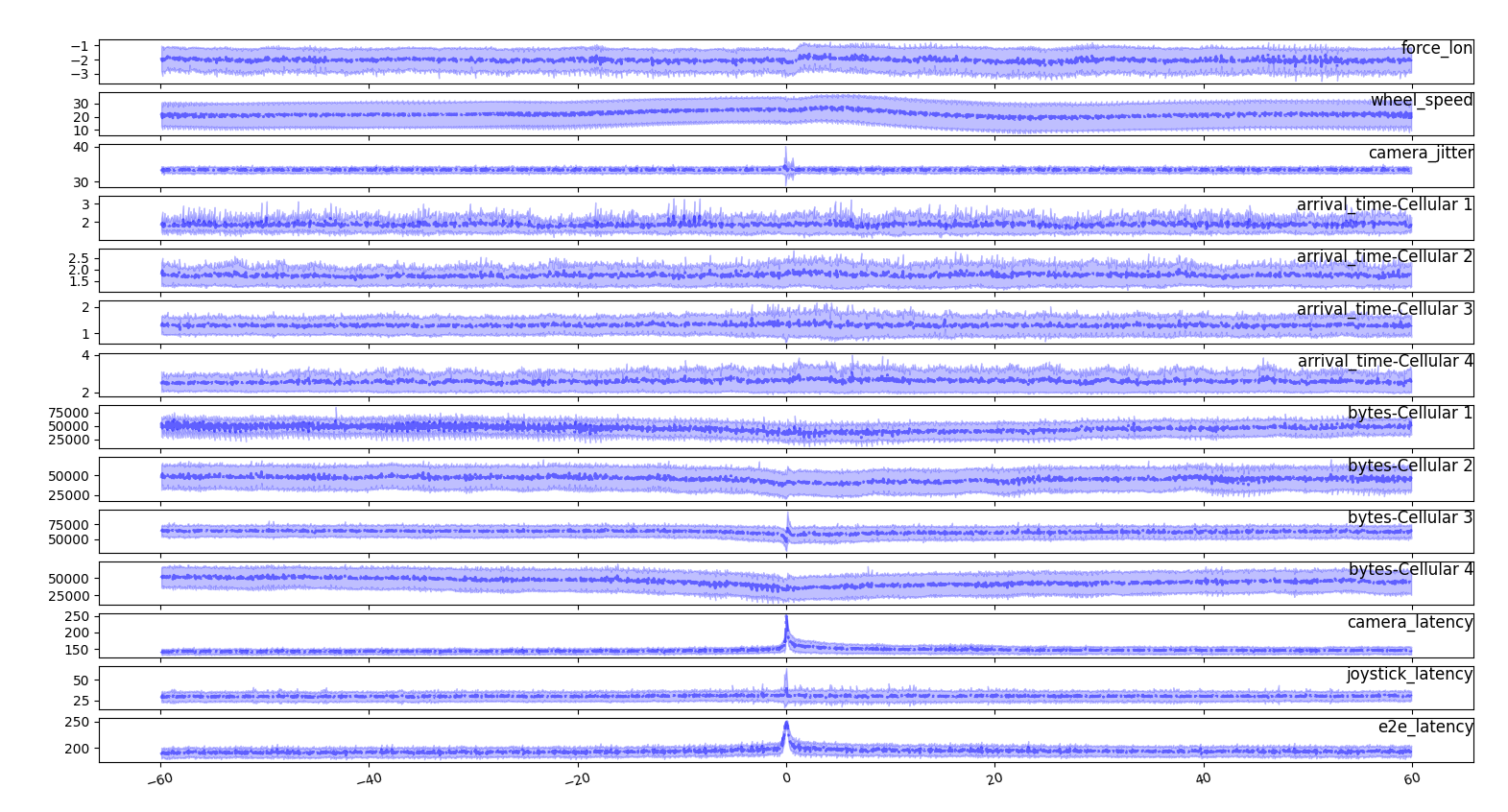 time
series on deci seconds
If we look at the few seconds close to the spike we don’t see clear signs of incoming spikes
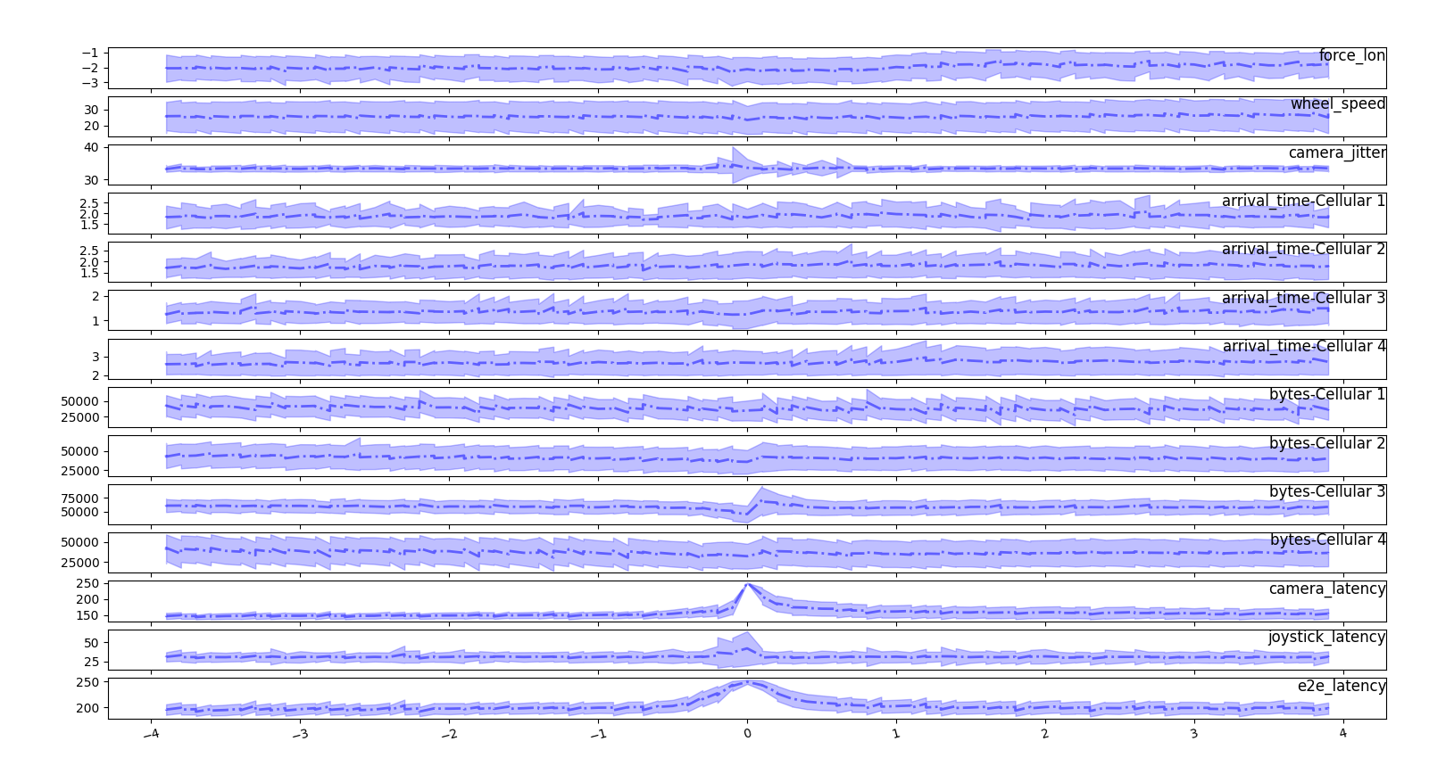 time series on deci seconds, detail
Neither looking at the derivative we see a clear trigger
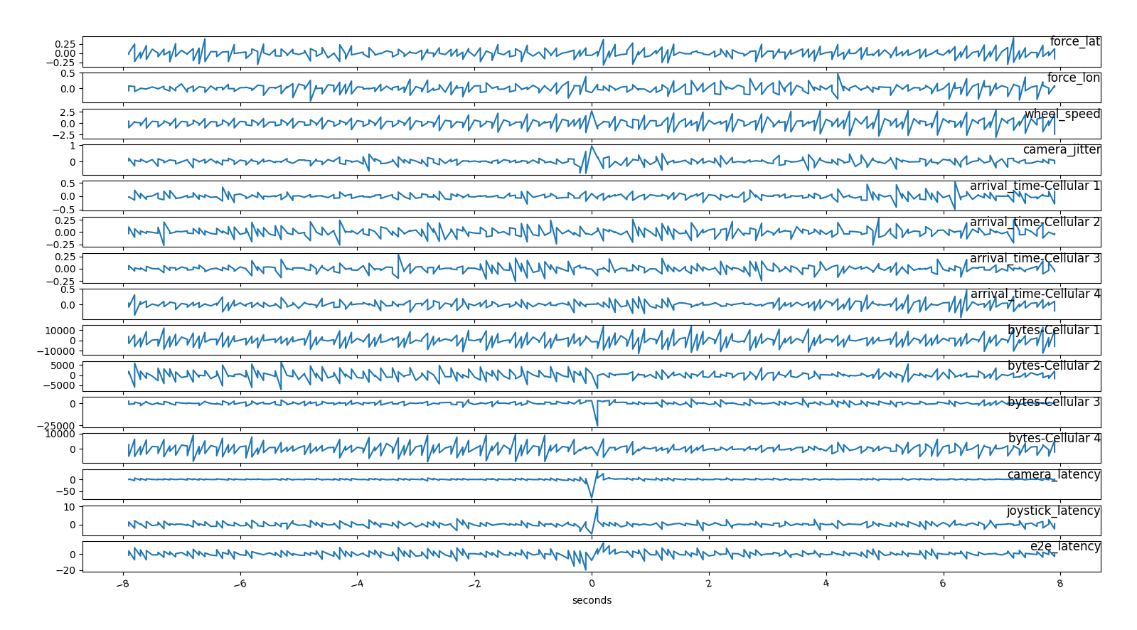 time series on deci seconds, derivative
We than smooth the series to have a better picture and start recognizing some patterns
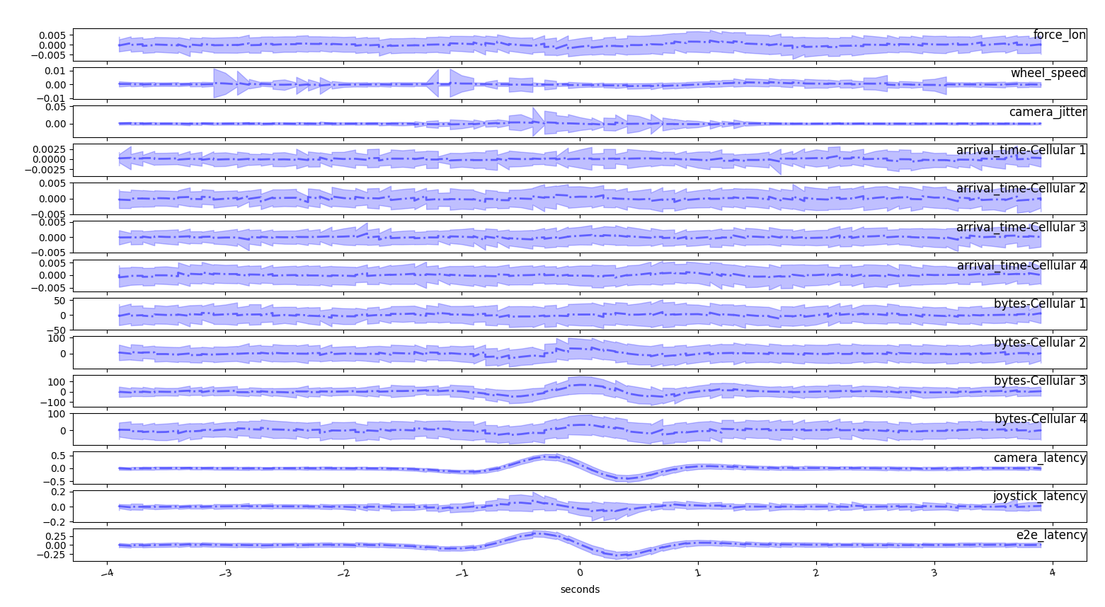 time series derivative on deci seconds, smoothed
