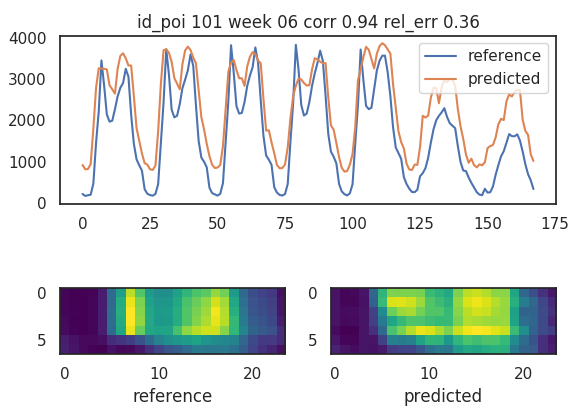
The code is a single script (script/etl.py) that uses the library lernia for machine learning and albio
For the current assessment we sketch an analysis procedure and we refer to a more detailed documentation on similar past use cases:
First of all we visualize the time series
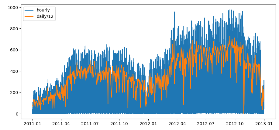 visualization of the time series for the hourly and daily resolutions
We than check data consistency:
| check | result |
|---|---|
| NaN | 0 |
| casual + registered == cnt | yes |
| suspicious missing atemp | 2 |
| suspicious missing windspeed | 2180 |
| suspicious missing hum | 22 |
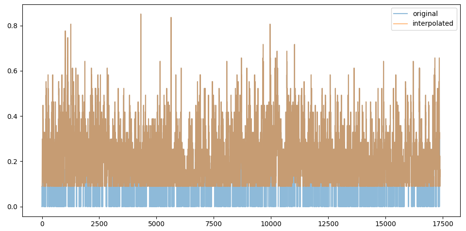 interpolating missing values for windspeed
The zero values for windspeed look like missing values, they represent 1% of the total values bu we decide to interpolate them nevertheless and we see that we slightly increase the overall correlation by replacing them.
We classify the features into two groups, continuous and categorical for running different type of tsts. For the continuous variables we can perform regression, and calculate metrics like information gain, relative error, , correlation…
Continous features are: temp, atemp, hum, windspeed,weathersit
For categorical features we can’t suppose that the values are ordered. Even for weathersit we don’t know if the ordering is monotonously correlating with the outcome.
We can turn categorical variables into continuous by stretching intervals, resorting values or grouping categories (for example grouping saturday and sunday into weekend for the varaible weekday). But in these case we will treat categorical variables separately.
Categorical variables are: mnth, hr, holiday, weekday, season, weathersit
The outcomes of the problems are: casual, registered, cnt
For continuous features we first calculate correlation to exclude the most obvious dependent features.
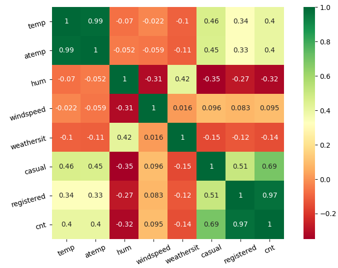 weather related features cross correlation
We clearly see that temp and atemp correlate and we keep atemp since contains more information(air humidity, windspeed…).
Since
cnt = registrated + casual
features correlate 100%, so we discard registered since is linearly dependent from the other two variables.
We don’t spot any other relevant correlation but we understand that humidity is a good predictor and most probably windspeed is not a good predictor and can be described by atemp and hum.
We check how categorical variables might subset the total count and we display the boxplot on the time variables
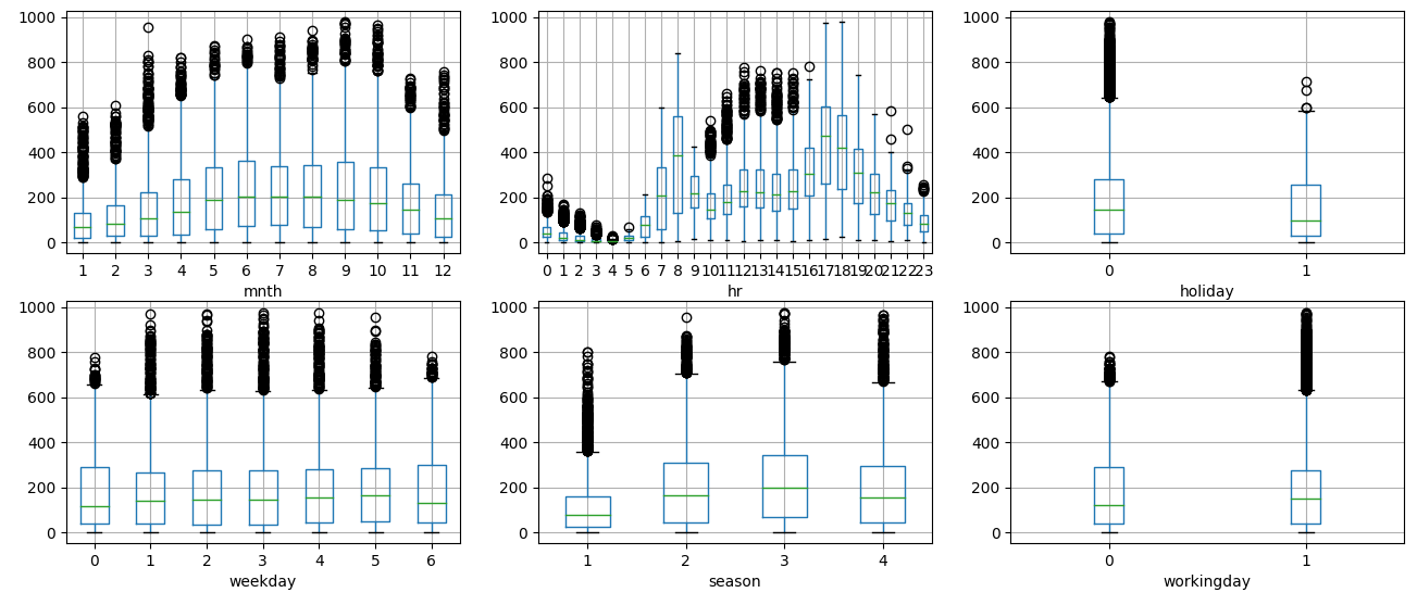 boxplot of
 cnt depending on time variables
We see that out of seven time variables only hr shows significant difference in counts, while the other variables show a light dependence on time.
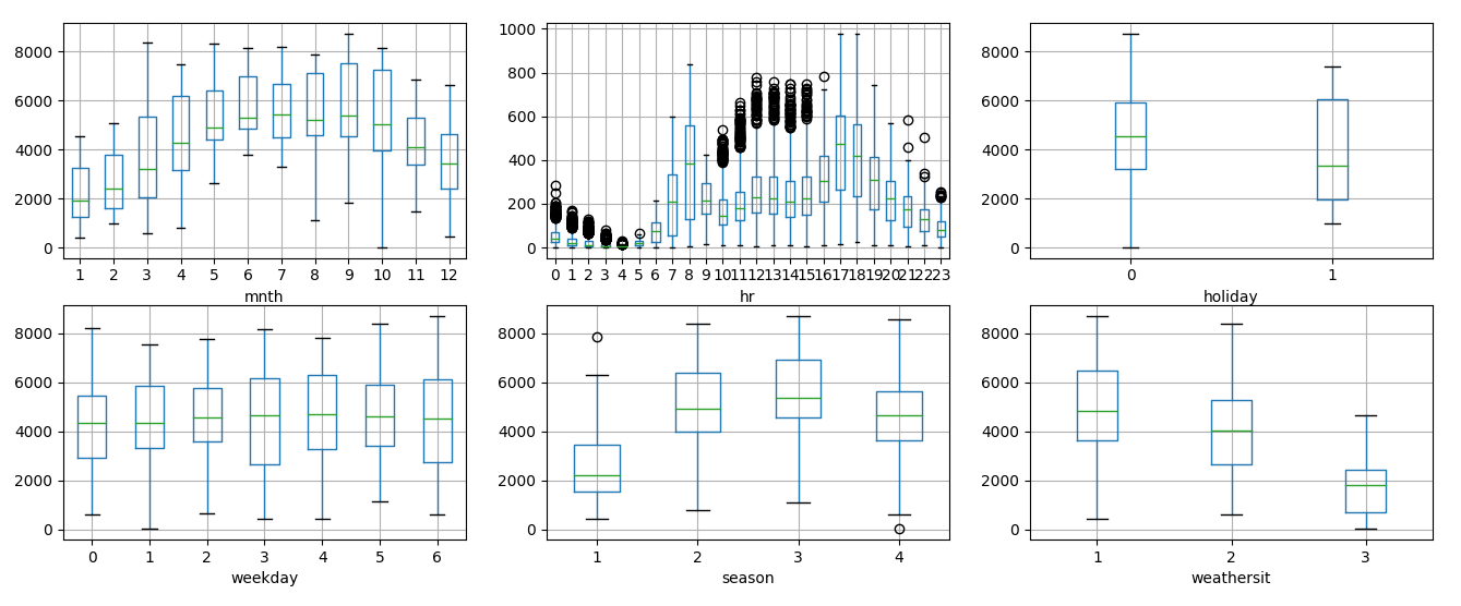 boxplot of
 cnt depending on time variables, daily values
Looking at the daily values we remove fluctuations and we see a clearer dependance with season and month
On the other side we can imagine how season and month correlate with temperature.
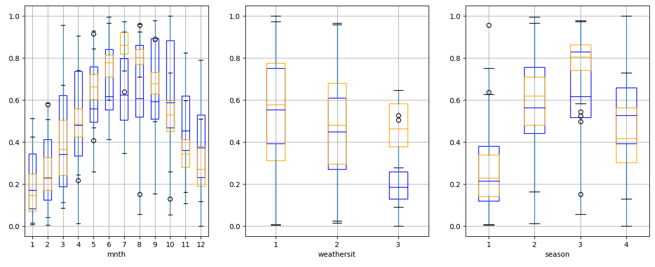 temperature (orange) and counts (blue) divided by time
Which means that the most information about the seasonal influence on counts is conveyed by temperature
Using hum, atemp, windspeed we can predict weathersit with 0.7 correlation.
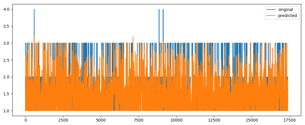 prediction of weather situation
Correlation is not high because cloudcover is not present.
weathersit is not well defined because values are bad distributed
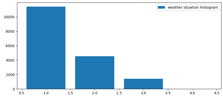 istogram
 weathersit
We than decide to not use it as predictor.
An important sign for predictor strenght is the variance analysis. We normalize the variables and display the variance.
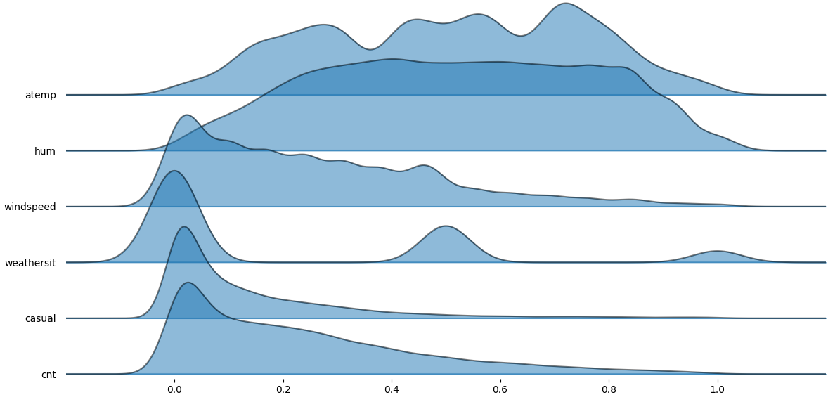 variance distribution
Big and small variances have bad prediction strength.
A different selection of features changes the relative weights.
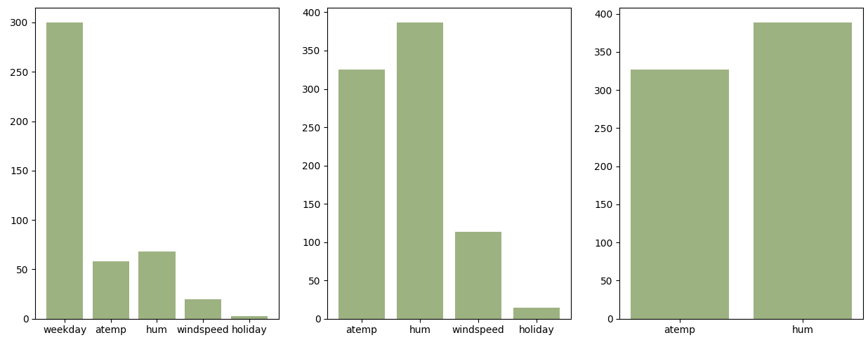 regression coefficients
We use a bagging regressor with an 6-fold cross validation taking random samples out of the series.
If we use atemp and hum we can predict cnt with reliable accuracy
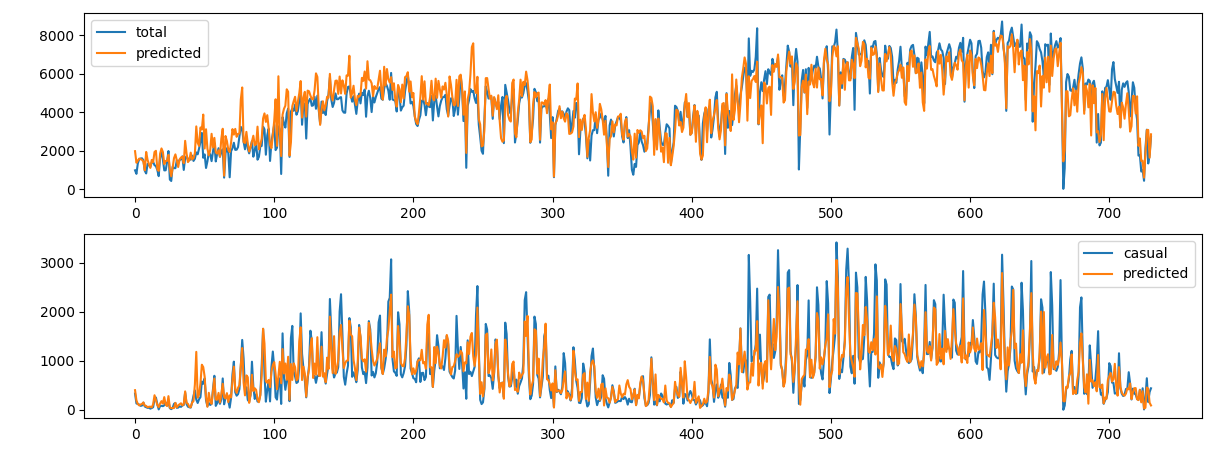 count prediction on daily values
| outcome | features | correlation | relative error |
|---|---|---|---|
cnt |
2 | 0.91 | 12 % |
casual |
2 | 0.87 | 24% |
cnt |
4 | 0.92 | 12 % |
casual |
4 | 0.94 | 15% |
Adding weekday and holiday improves only the performances for casual customers which is expected since recurrent customers have a more stable pattern.
The regular structure is easily predicted by the regressor.
To predict the hourly values we divide the daily sum by the hourly split and have a regular pattern to predict. We remove weather features and train with hr, weekday, and holiday.
We do a 10-fold cross validation with the same bagging regressor.
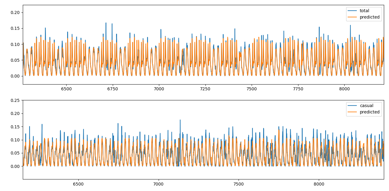 count prediction on hourly values
| outcome | features | correlation | relative error |
|---|---|---|---|
cnt |
3 | 0.92 | 15 % |
casual |
3 | 0.83 | 29% |
If we pipe together the two predictions we achieve good correlation and acceptable relative error.
| outcome | features | correlation | relative error |
|---|---|---|---|
cnt |
3 | 0.92 | 23 % |
casual |
3 | 0.91 | 30% |
To forecast half of the remaining day we sum only the first 12 h of the day to predict the daily values.
 prediction with half day info
| outcome | features | correlation | relative error |
|---|---|---|---|
cnt |
3 | 0.79 | 60 % |
We can further improve the results calculating the correct ratio between the two parts of the day and perform a separate prediction for the two half of the day.