We create a mapping based on some reference data referring to a small geographic area we can’t resolve with our data.
explanation on capture rate
We don’t know a priori how each cell contributes to the measurement of visitors and we create an iterative process to estabilsh the contribution of each cell.
Reference data have internal consistency that varies from location to location.
We first control how stable is the correlation adding noise.
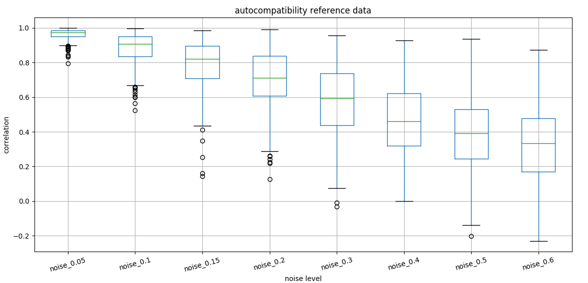 stability of correlation introducing
noise
We can show as well that noise at the hourly level does not change correlation as fast as for daily values.
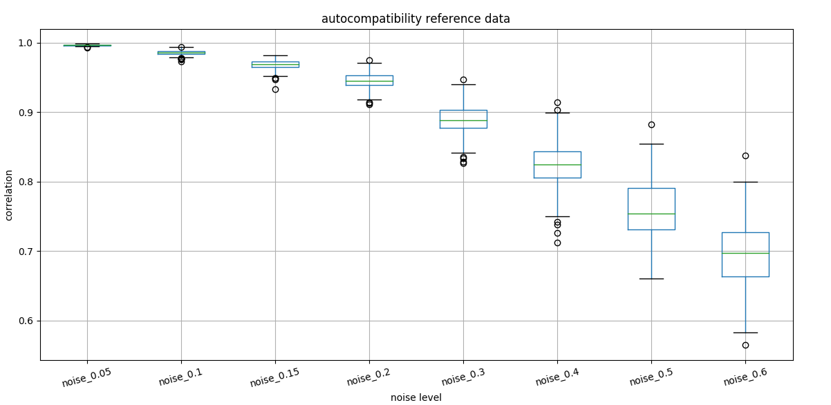 noise on reference
data
We see the effect of noise on reference data
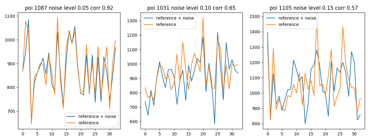 noise on reference data
Already with 15% noise we can’t match the reference data with correlation 0.6 at a constant relative error.
If we look at historical data (variance of days with the same isocalendar date) we see that holiday have a big contribution in deviation.
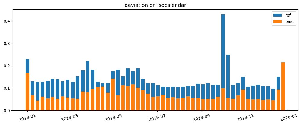 deviation on isocalendar
We quantify the forcastability of a customer time series running a long short term memory on reference data.
We can see that some reference data are easy forcastable by the model
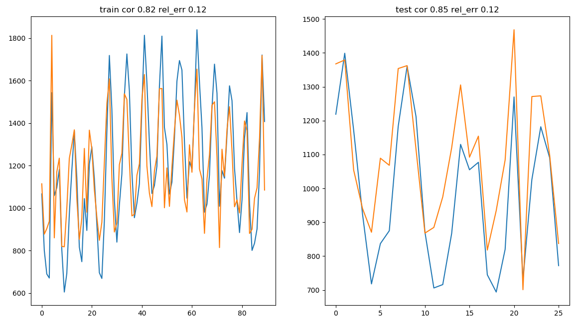 example of good forecastable
model
While some are not understood from the neural network
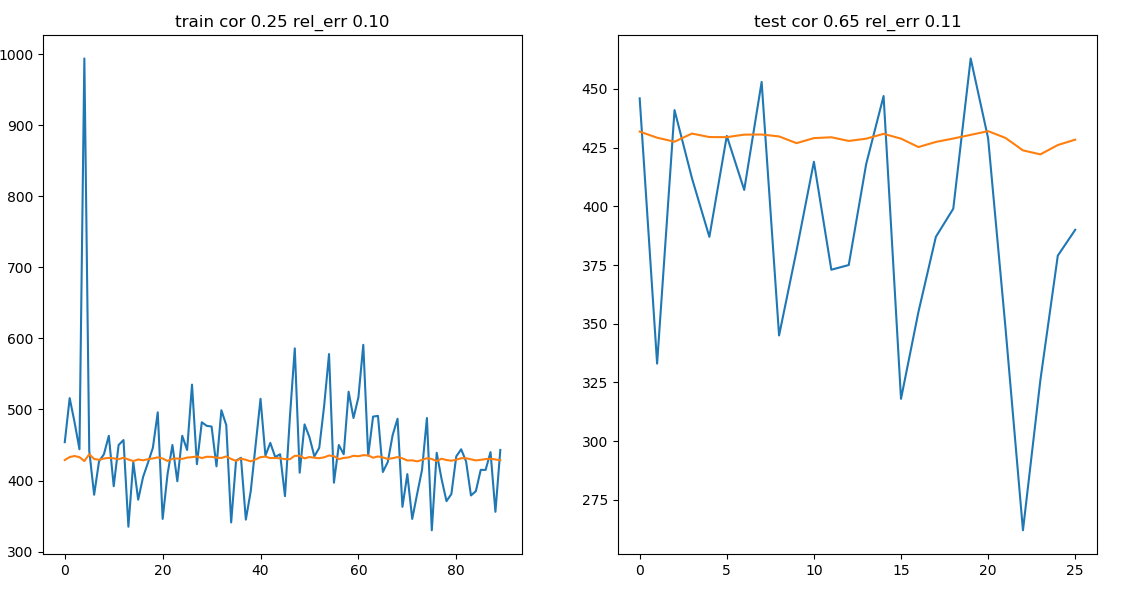 example of bad forecastable model
We use the following job file to produce the activity with the filters:
filter on activities
Filtering does not change the overall curves but just the niveau
Filtering options:
| name | tripEx | distance | duration | chirality |
|---|---|---|---|---|
| t4 | 10.5 | 20km | 30min-2h | True |
| t4_10 | 10.5 | 10km | 15min-2h | True |
| t4_p11 | 11.6 | 20km | 15min-2h | True |
| t4_p11_d20-notime | 11.6 | 20km | 15min-2h | True |
| t4_p11_d10 | 11.6 | 10km | 15min-2h | True |
| t4_p11_d20 | 11.6 | 20km | 15min-2h | True |
| t4_p11_d30 | 11.6 | 30km | 15min-2h | True |
| t4_p11_d40 | 11.6 | 40km | 15min-2h | True |
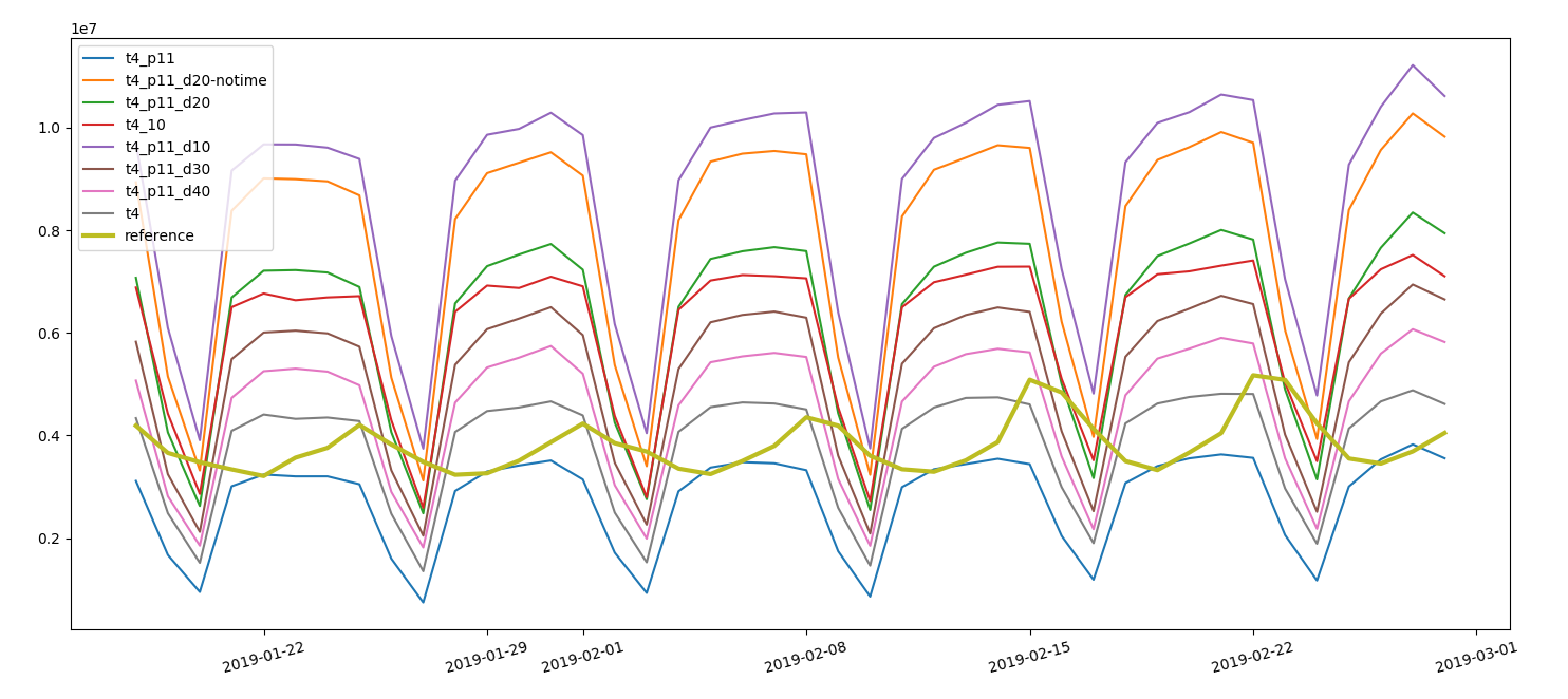 effect of
filters on curves
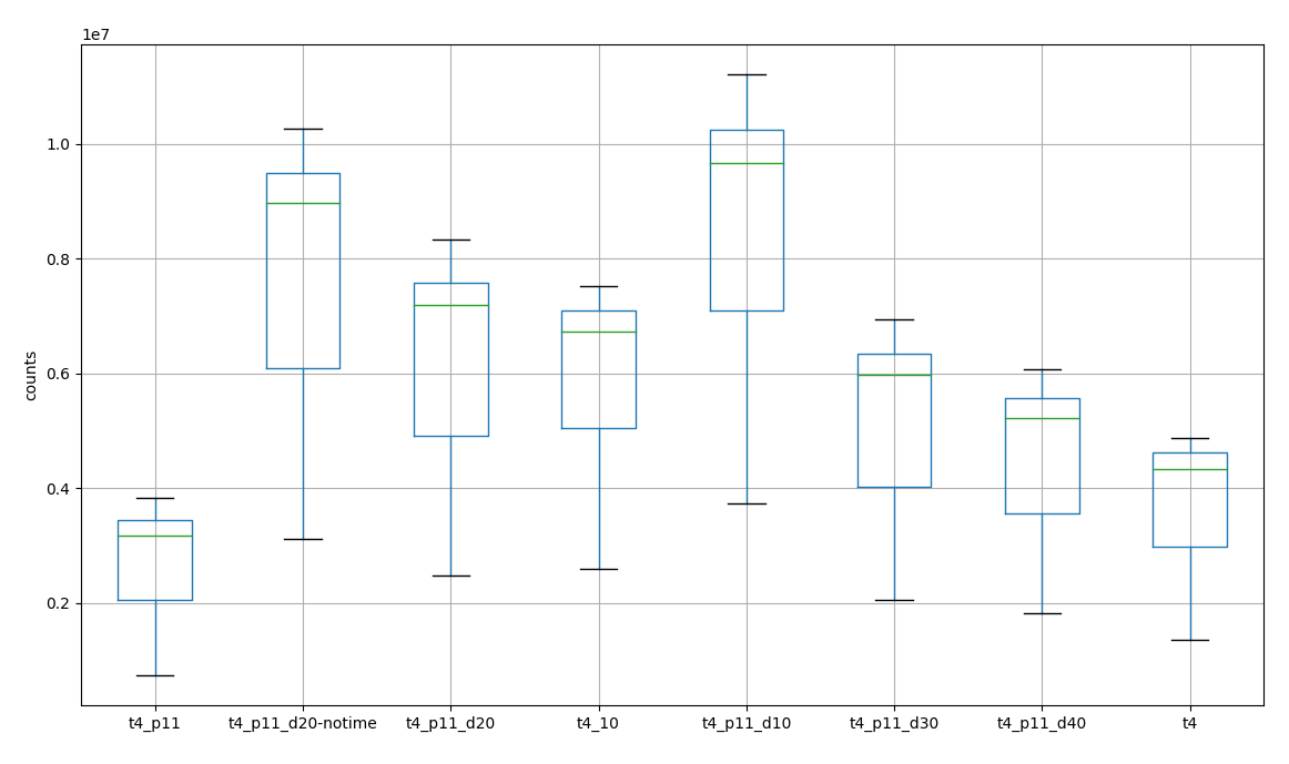 counts
changed by filtering
We calculate daily values on cilac basis.
The tarball is downloaded and processed with an etl script which uses the a function to unpack the tar and process the output with spark.
We filter the cells using only the first 20 ones whose centroid is close to the poi.
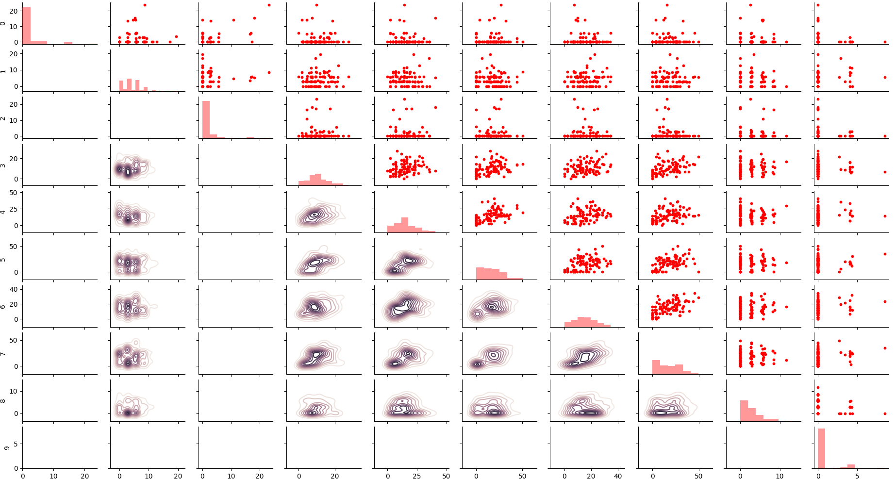 some
cells are not correlating within each other
At first sight the sum of activities doesn’t mirror the reference data, neither in sum nor in correlation.
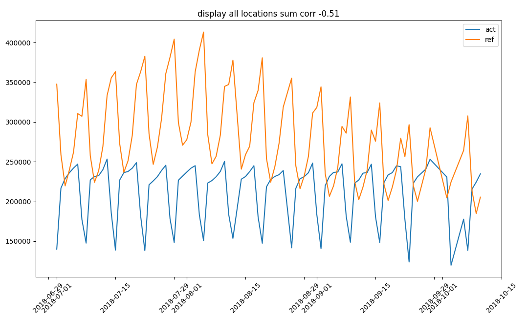 sum of overall activities and visits
We use linLeastSq to find the best linear weights for each cell contributing to measure the activities at the location.
   def ser_sin(x,t,param): #weights times activities
        return x*t.sum(axis=0)
    def ser_fun_min(x,t,y,param): #minimizing total sum
        return ser_sin(x,t,param).sum() - y.sum()
    x0 = X.sum(axis=0) #starting values
    x0 = x0/x0.mean() #normalization
    res = least_squares(ser_fun_min,x0,args=(X,y,x0)) #least square optimization
    beta_hat = res['x']
function that optimizes cells weights minimizing the total sum difference wrt reference data
We iterate over all locations to find the best weight set using a minimum number of cells (i.e. 5)
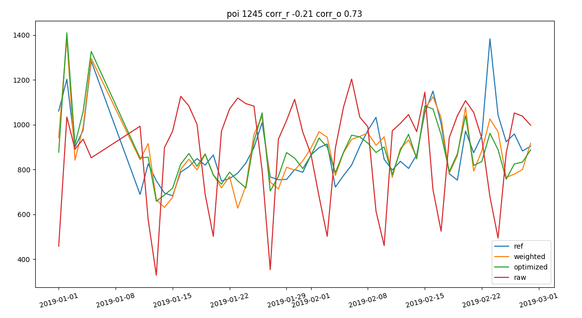 linear regression on
cells
We iterate over the different filters and we see a slight improvement in input data which is, on the other hand, irrelevant after weighting.
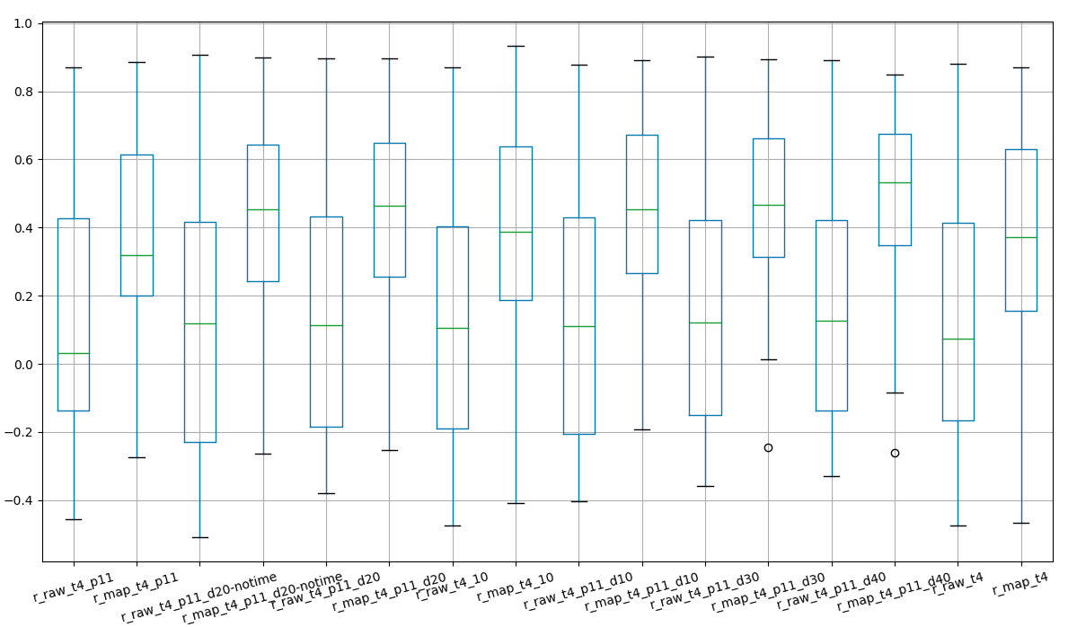 effect of
filtering on correlation pre and post mapping
Among all the different combination we prefere the version 11.6.1, 40 km previous distance, chirality, 0 to 2h dwelling time.
We see that chirality is stable but a third of counts doesn’t have a chirality assigned.
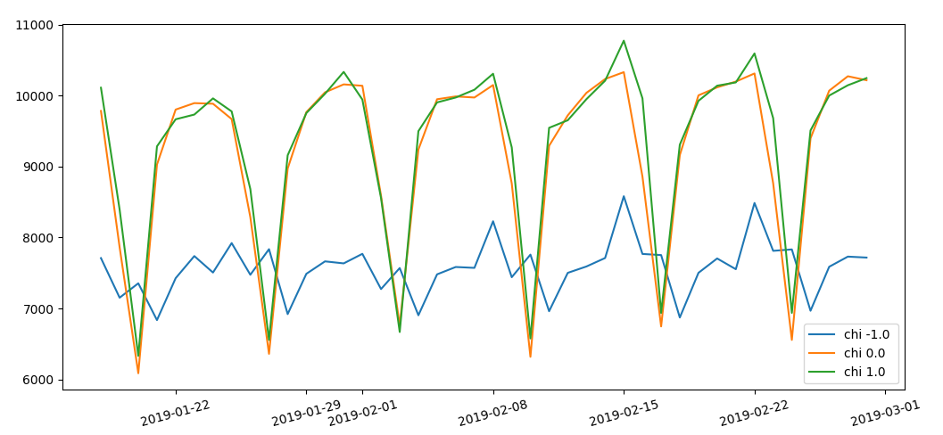 daily
values of chirality
We monitor the effect of the different steps on the total correlation with reference values.
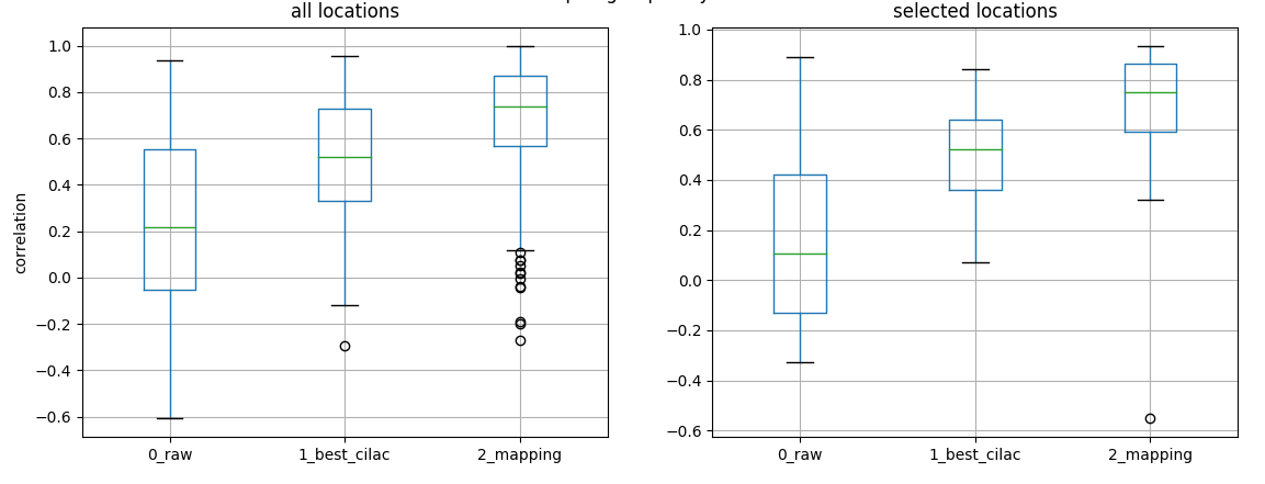 correlation monitorin after any process
step
We use etl_dirCount to download with beautifulSoup all the processd day from the analyzer output and create a query to the postgres database.
A spark function loads into all the database outputs into a pandas dataframe, take the maximum of the incoming flow and correct the timezone.
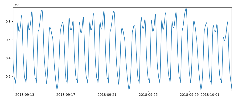 direction counts
Now we check the stability of the capture rate over time and the min-max interval on monthly and daily values.
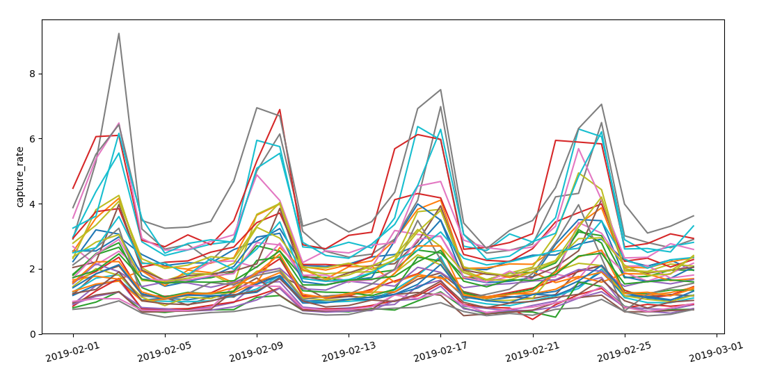 capture
rate over different locations which show a common pattern
We see that the range of maximum and minimum capture rate is similar over different locations and we don’t have problematic outliers.
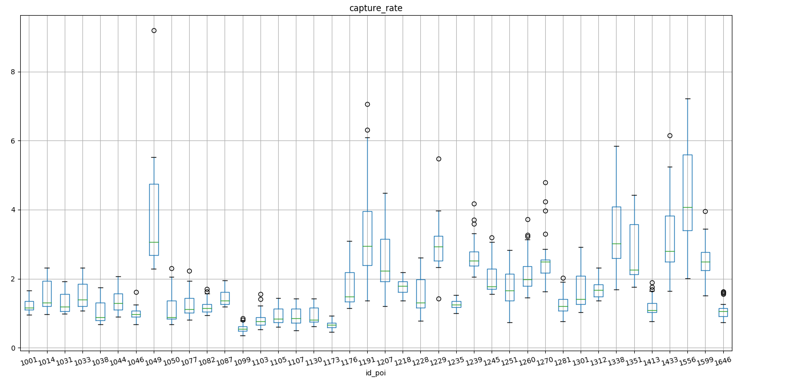 capture rate
boxplot over different locations
Over the time different models were tested to select the one with the best performances and stability.
The suite basically consists in:
We use learn_play to run a series of regressor on the time series.
Depending on the temporal resolution we use a different series of train_execute
We use kpi_viz to visualize the performances
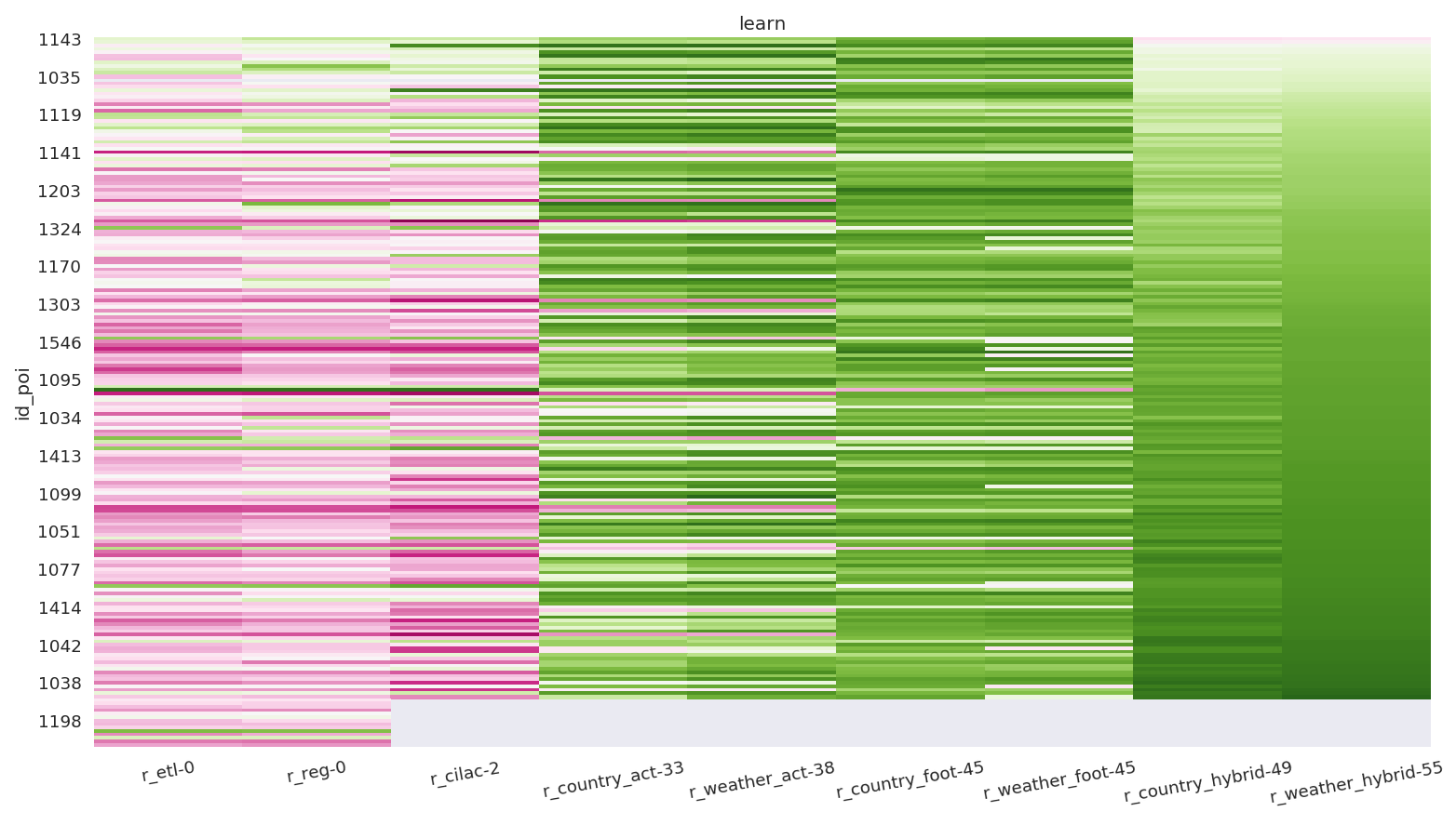 kpi boost
We prepare a dataset overlapping the following information:
We can see that not only all data sources are presents
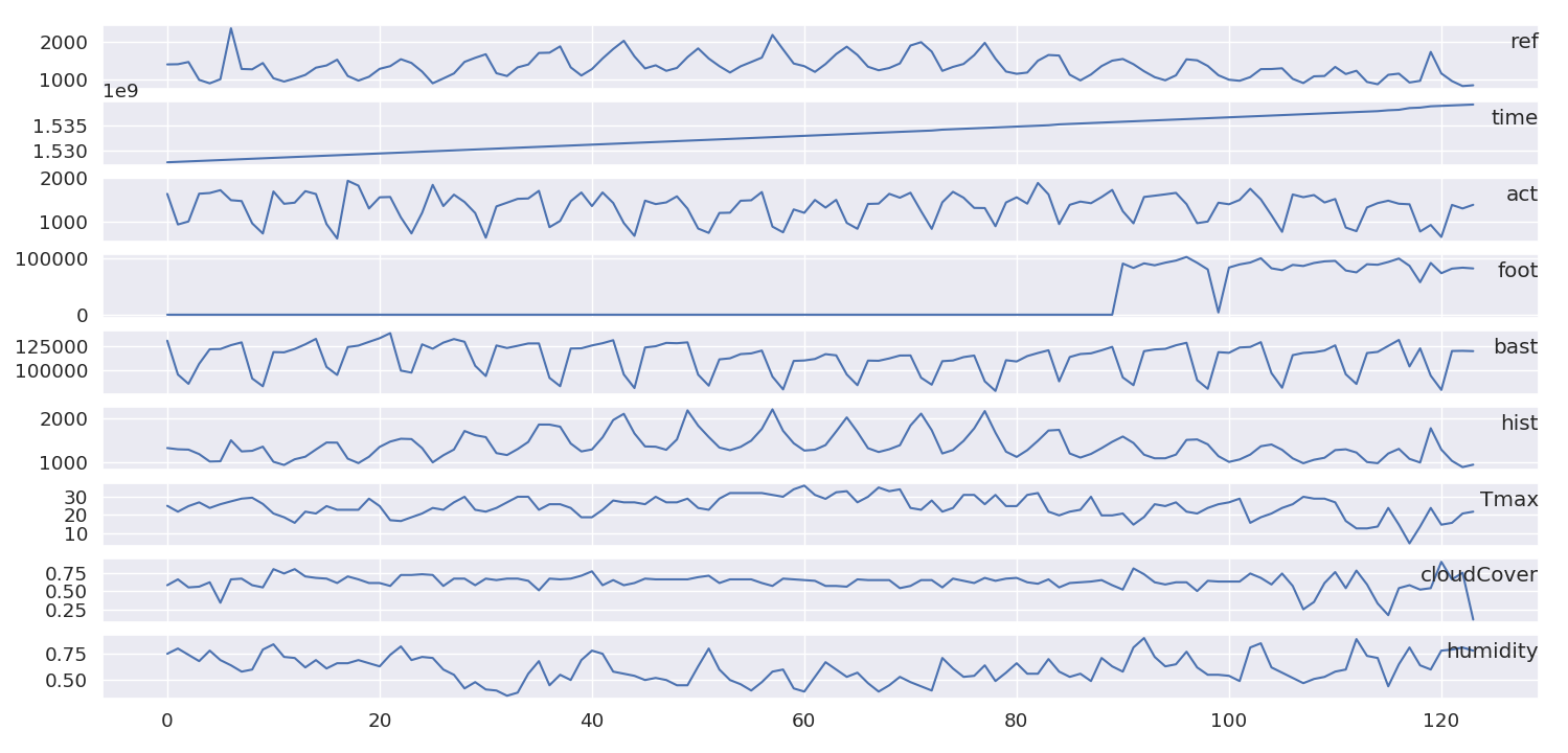 input data
We than iterate over all locations and run a forecast over 30 days using a long short term memory algorithm train_longShort
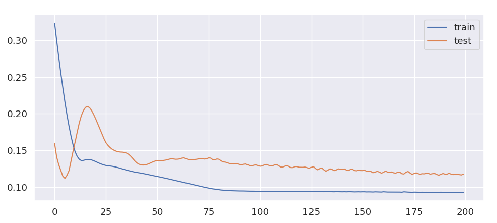 performance history
We can see that the learning curve is pretty steep at the beginning and converges towards the plateau of the training set performance.
We start preparing the data for a first set of location where:
We summarized the most important metrics in this graph
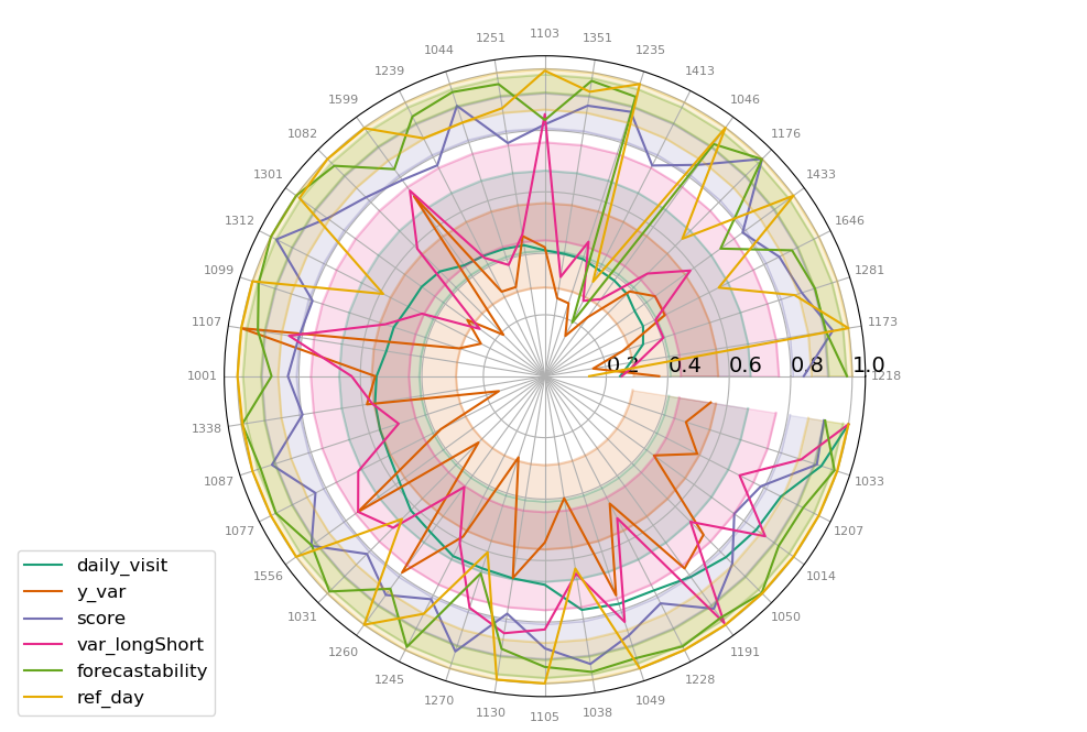 range of scores, relative values, 0 as minimum,
areas represent confidence interval
and summarized in this table.
Performances depend on the regularity of input data over time.
The cooperation with insight is required for:
TODOs:
After the finalization of the prediction of the reference data another prediction model has to be built to derive motorway guest counts for competitor locations.
This model will take into consideration:
