Restaurant Guests

Our scope is to predict restaurant guests from telco data.

deriving capture rate from footfall und activities

The underlying model can be described as

g_receipts(t)../f/f_{people/receipt}(t) = c_rate^a(t)a_act(t)f_ext + c_rate^f(t)a_foot(t)f_ext + b_bias(t)

Where activities and footfall are not independent.

We have to understand the underlying relationship between telco data and reference data.

Use case description

Each commercial activities that capture a fraction of the users passing by. The quote of users capture by the activity depends on:

• Type of activity
• Advertising
• Capacity
• Parking places
• Type of street
• …

How exactely the capture rate depends on the specific location features is going to be investigated by training a prediction model.

Procedure

We will proceed in the following way:

• enirch location information with all the available information we have (public statistical data)
• we define and calculate the score
• we extract and process direction counts
• we create a sensor specific mapping per location
• we iterate the regressor on activities and direction count to match customer data

Data enrichment

Degeneracy

Degeneracy is a measure of sparsity or replication of states, in this case we use the term to define the recurrency of pois in a spatial region.

The operative definition is to calculate the distribution of other pois at a certain distance. To reduce the complexity of the metric we perform a parabolic interpolation and define the degeneracy as the intercept of the parabola fitting the radial density distribution.

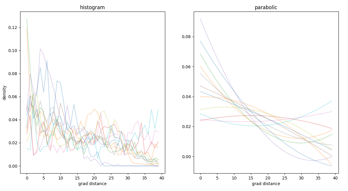spatial degeneracy, only the intercept is taken into consideration

Population density

We enrich poi information with official statistical data like:

• population density
• men/women asymmetry
• foreigner percentage
• flat density
• land use
• age asymmetry

We don’t know a priori which parameter is relevant for learning and we might have surprisingly perfomances from features that do not seem to have connection with the metric.

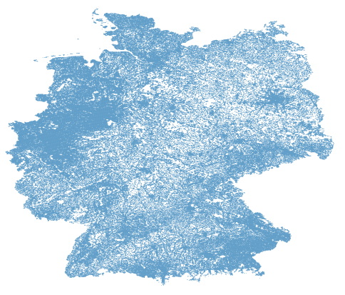distribution of official census data

To obtain the value of population density we interpolate over the neighboring tiles with official census data using a stiff multiquadratic function.

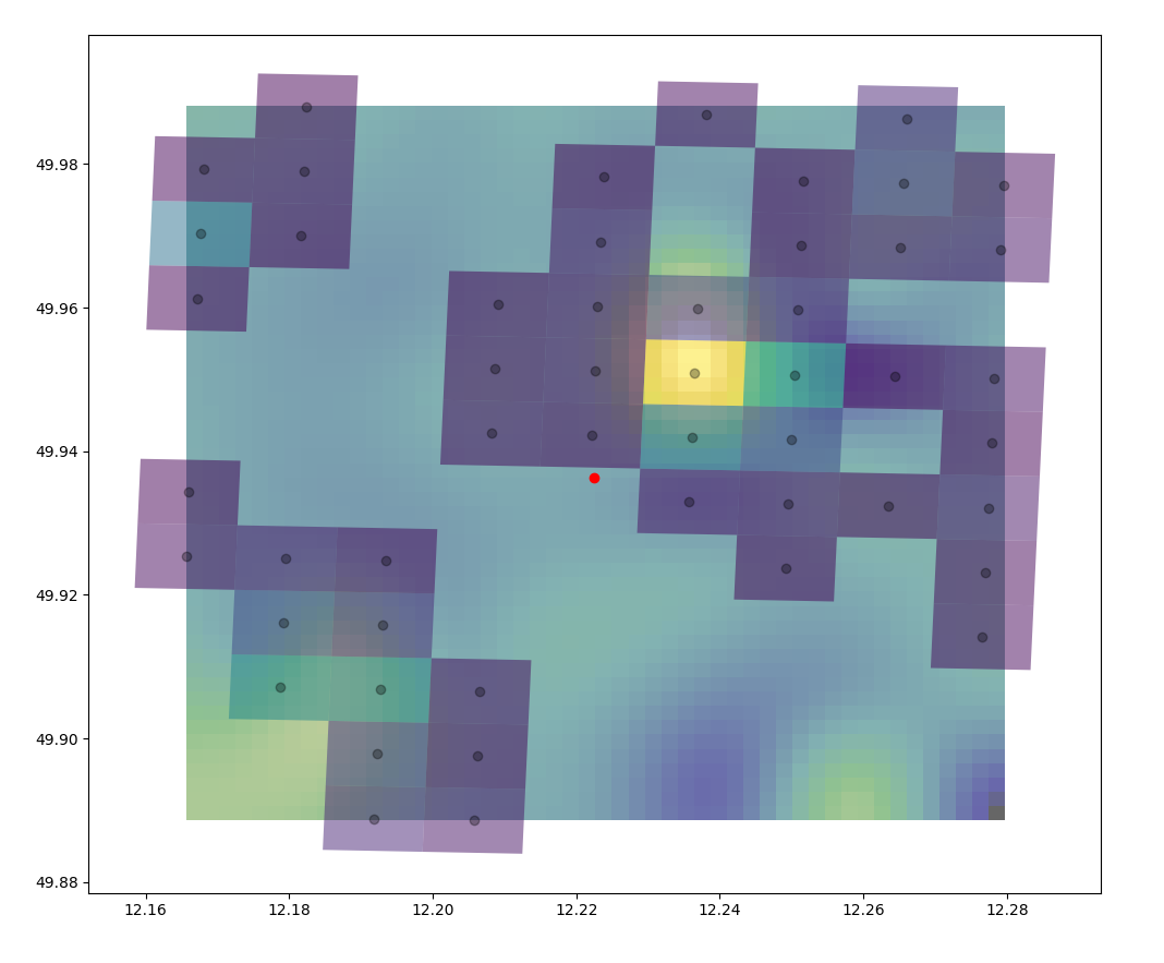determination of the density value coming from the neighboring tiles of the official statistics

Isochrone

For each location we download the local network and calculate the isochrones

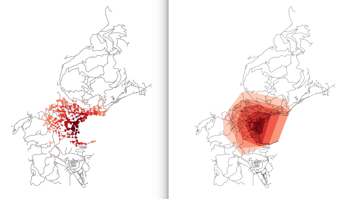isochrone, selected nodes and convex hulls

Footfall

On a regular grid over the whole country we route all the users across the street and associate a footfall count to each tile crossing that street.

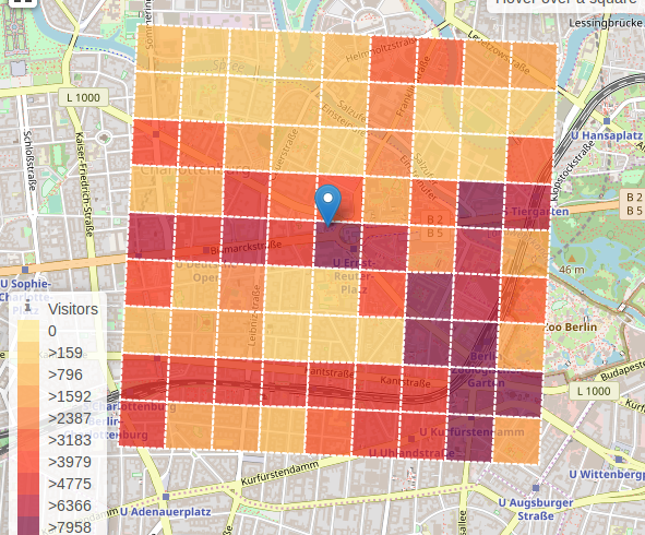footfall over the tiles per hour and day

Other metrics

We enrich the location information with street statistics

• Bast counts: number of cars measured in the closest street
  • bast
• Bast weekend factor: correction factor between workdays and weekdays, distinguish between commuter and touristic stretches
  • bast_fr, bast_su: correction factors for friday and sunday

Time series preprocessing

We see anomalous peaks and missing points in reference data which we have substituted by the average

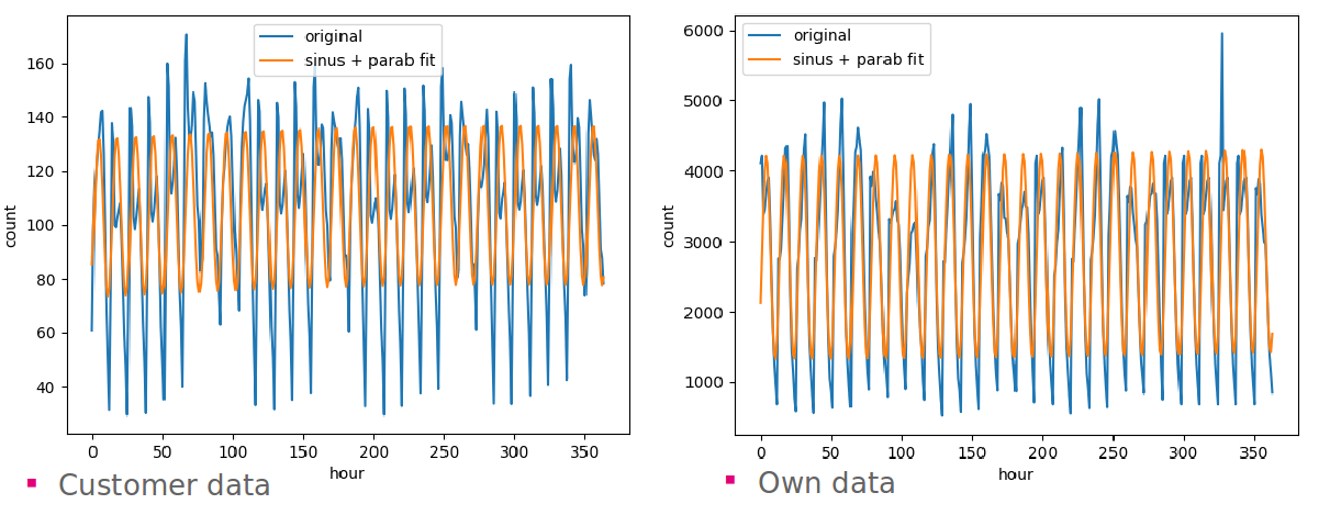hourly visits and footfalls over all locations

We can see that the main difference between in the daily average is the midday peak

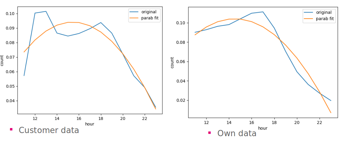daily visits and footfalls over all locations

Customer data are more regular than footfall data

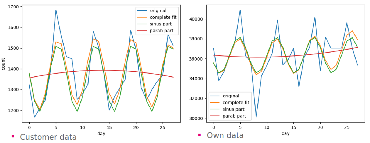total daily visits and footfalls over all locations

We create a matrix representation of the input data to speed up operations 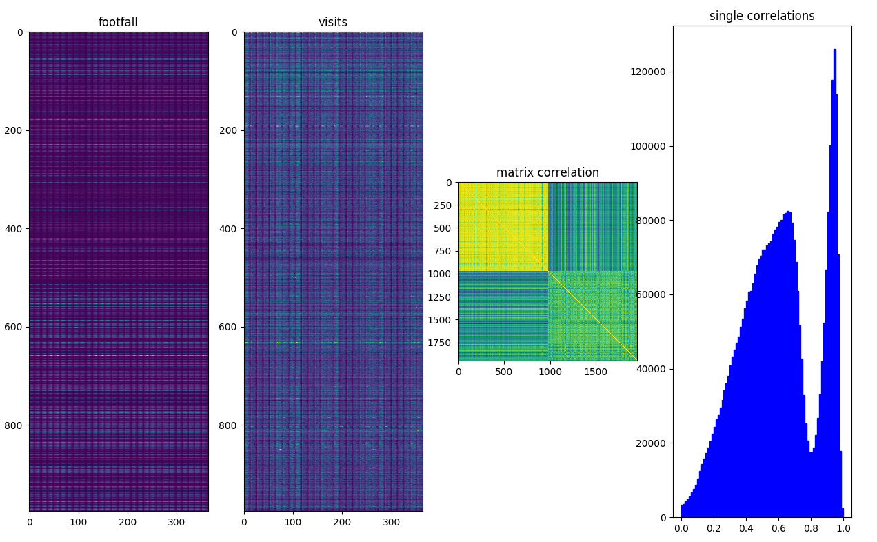matrix representation of footfall and visits and their mutual correlation

sensor mapping

We calculate daily values of activities per sensor and we use correlation as scoring to understand how the influence of neighboring sensors can describe visitors.

We first calculate sensor cross correlation and keep only consistent sensors

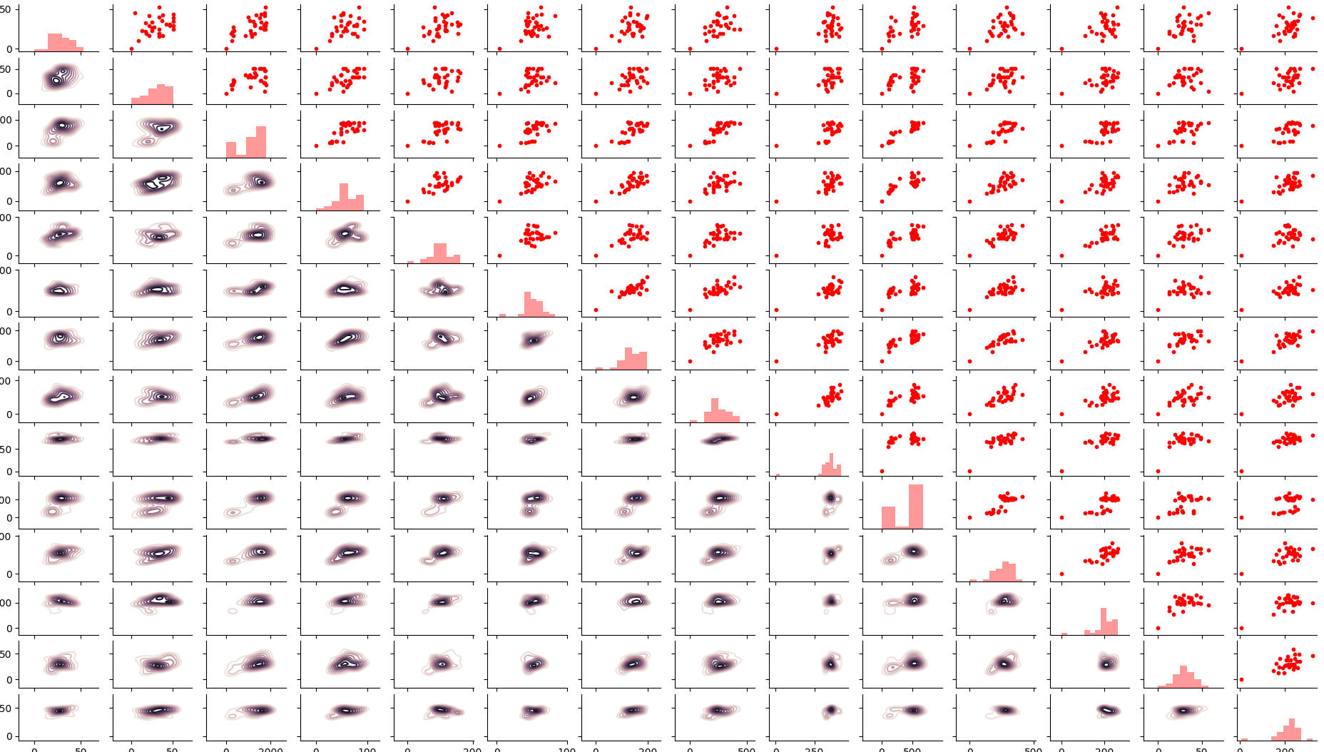sensor cross correlation

We than run a regression to estimate the weighting of the sensor activities versus visits. We filter out the most significant weight and we rerun the regression.

We do a consistency check and cluster the cells as restaurant activities.

If we consider all sensor with weight 1 we score 11% (of the location over 0.6 correlation) 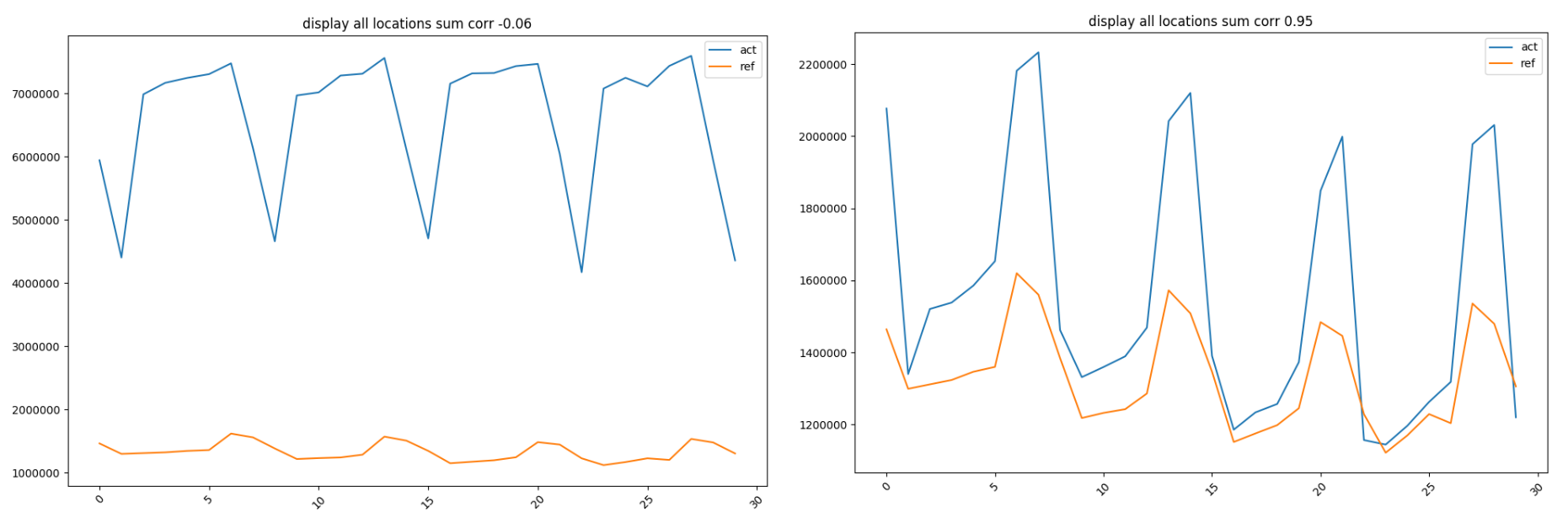unweighted and weighted sensor mapping

If we weight all sensors performing a linear regression we score 66%

KPI

We calculate the first score, _cor, as the Pearson’s r correlation: $$ r = \frac{cov(x,y)}{\sigma_x \sigma_y} $$

We calculate the relative difference as: $$ d = 2\frac{\bar{x}-\bar{y}}{\bar{x}+\bar{y}} $$

And the relative error as: $$ s = 2\frac{\sqrt{\sum (x - y)^2}}{N(\bar{x}+\bar{y})} $$

We have few location where footfall correlates with visitors and we don’t see a clear dependency between scoring and location type.

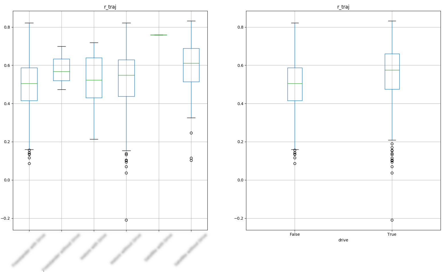boxplot foot_vist

If we consider daily values activities and footfall don’t correlate at first with reference data.

performances over sources

Activities and footfalls have a good correlation.

Regression

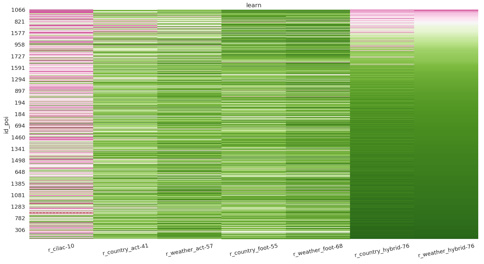
We perform a regression of measured data versus reference receipts and we calculate the performance over all locations.

The first regressor is country wide, the second is site type specific:

• maps the sensors giving a specific weight (bayesian regressor)
• groups the sensors and sum up the activities for the specific location - performance 10%
• country wide regressor on activity - performance 41%
• location type specific regressor on activity- performace 57%
• country wide regressor on footfall - performance 55%
• location type specific regressor on footfall- performace 68%
• country wide regressor on hybrid - performance 76%
• location type specific regressor on hybrid- performace 76%

performance over iterations

We can see that an hybrid model is the best solution to cover 3/4 of the locations.

Feature selection counts

We have collected and selected many features and we have to simplify the parameter space: 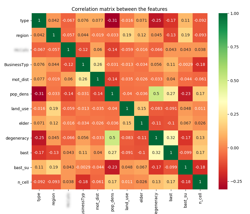correlation between features

We select the features which have the higher variance. 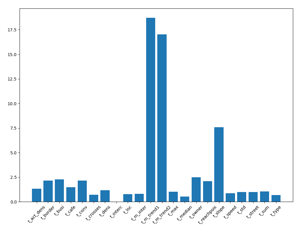relative variance of single features

We can see that the selected variances are mutally well distributed 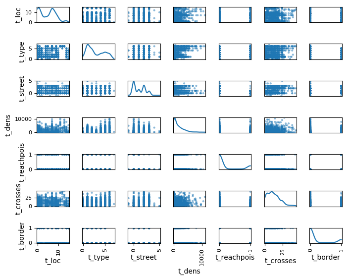mutual distribution of selected features

Features knock out

We are interested in understanding which time series is relevant for the training of the model. To quantify feature importance instead of using a different model that returns feature importance (like xgboost or extra tree classifier) but might not correspond to the importance of the real model we just retrained the model removing each time one of the feature.

First we fix pair of locations (one train one test) and we retrain the models without one feature to see how performances change depending on that feature.

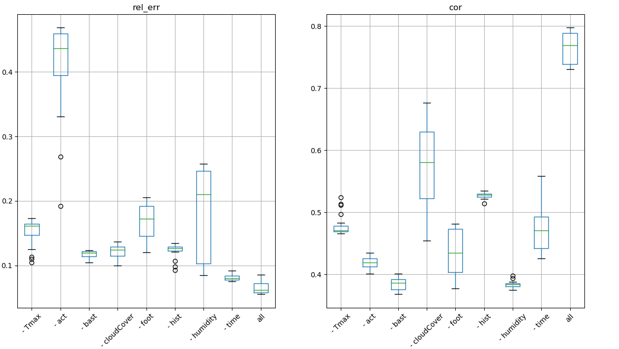feature importance on performances, fix pair

If we train on one location and we test on a different random location we don’t have stable results to interpret

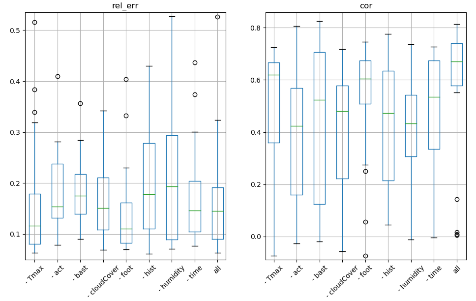feature importance on performances

Prediction on daily visits

We want to predict the number of visits based on pure geographical data by running a regressor with cross validation

reference vs prediction

Now we have to iterate the knowledge over unknown locations.

Time series prediction

We use a long short term memory with keras to create a supervised version of the time series and forecast the time series of another location.

We use train_longShort to load and process all the sources.

For each location we take the following time series shifting each series by two steps for the preparing the supervised data set.

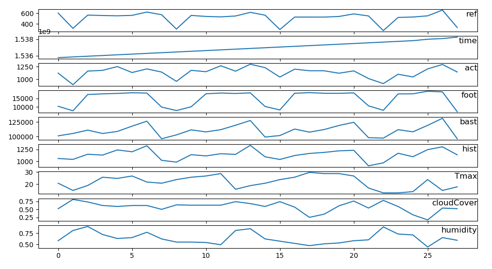set of time series used

We can see that in few epochs the test set performance converges to the train set performance.

• Training time: 8 min

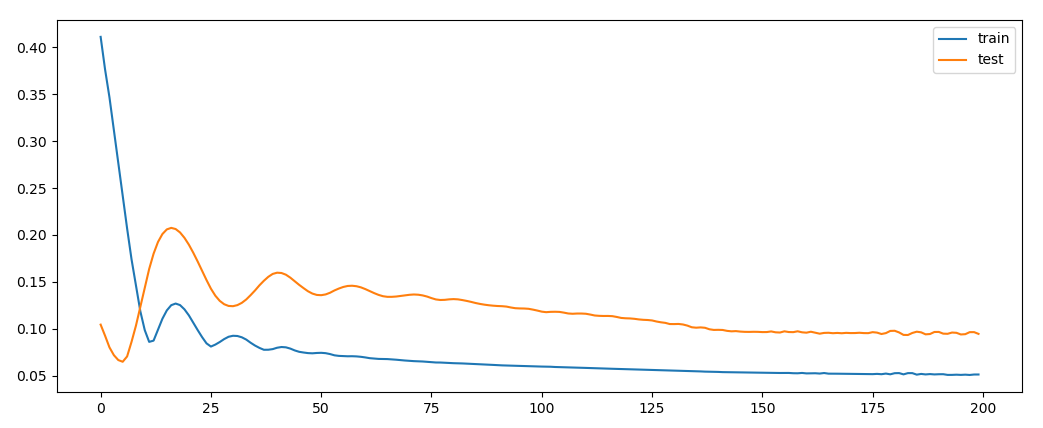learning cycle

The test group consists in a random location taken within the same group. We see that performances don’t stabilize over time but rather get worse which depends on the type of location as we can see later.

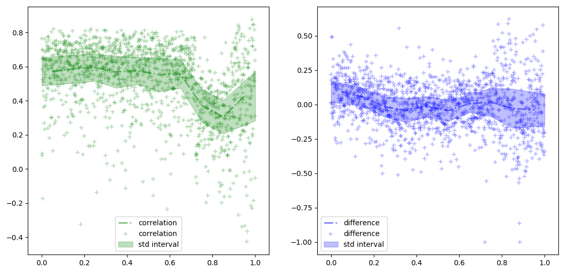score history

Overall performances are good for relative error and relative difference for correlation we will se that performances are strongly type dependent.

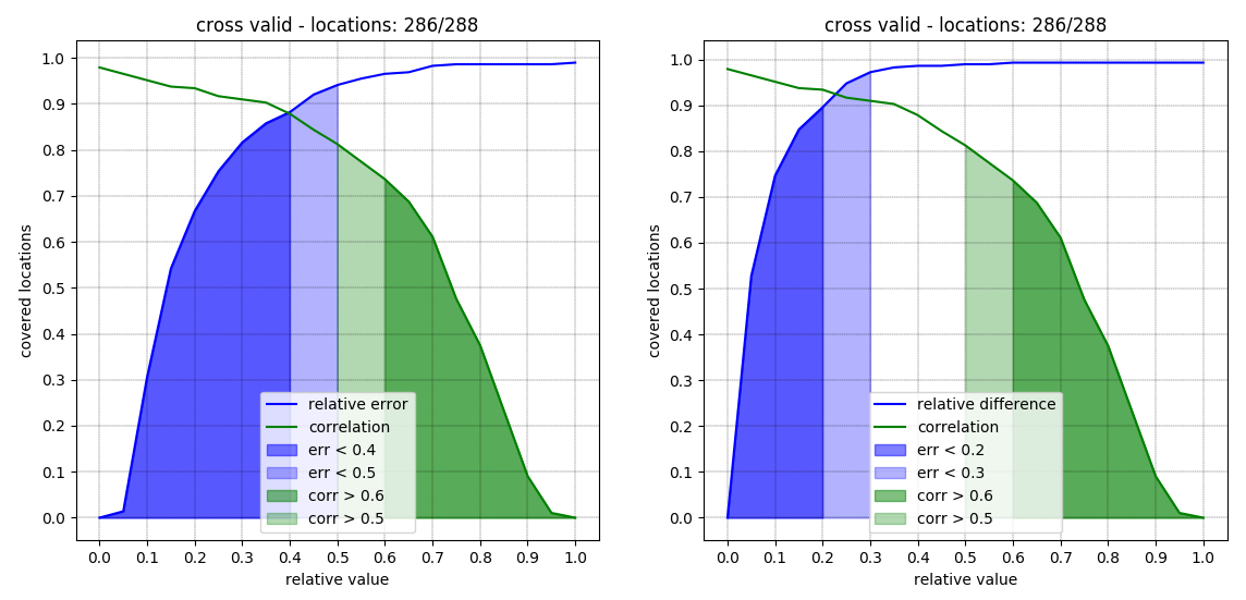kpi for fixed validation set

A fix validation set is not necessary since performances stabilizes quickly over time.

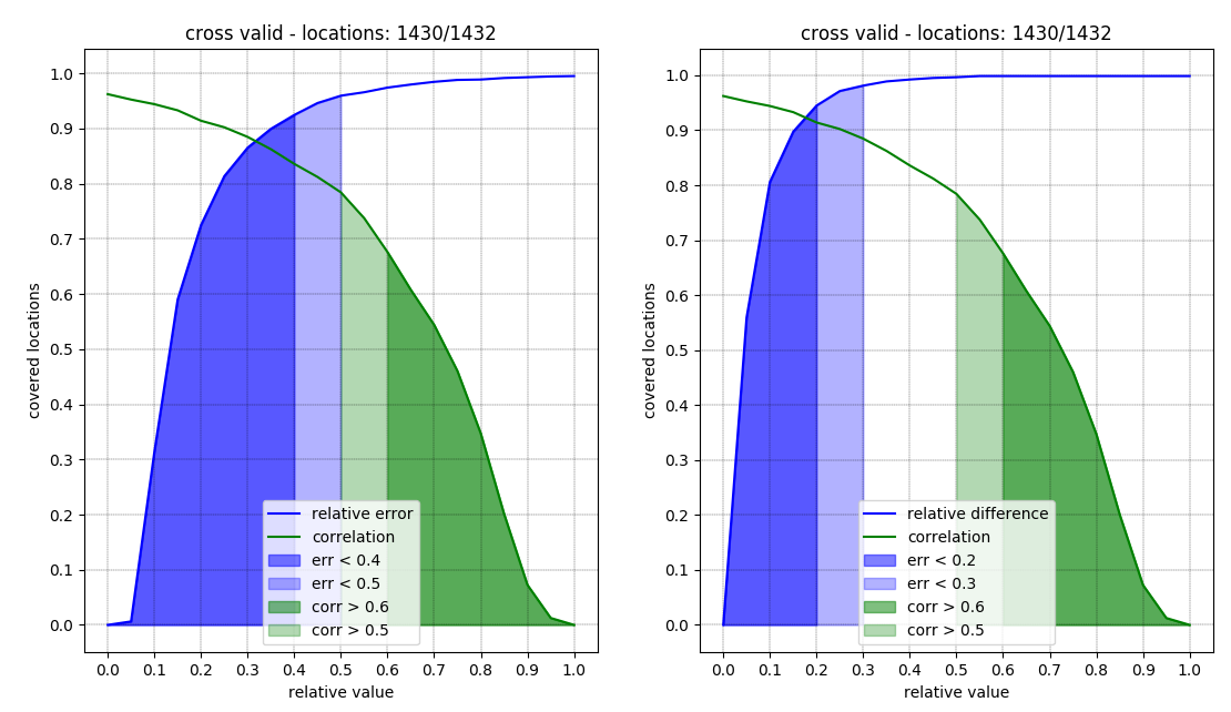kpi relative error and relative difference

Relative error as a regular decay while correlation has a second peak around 0.4

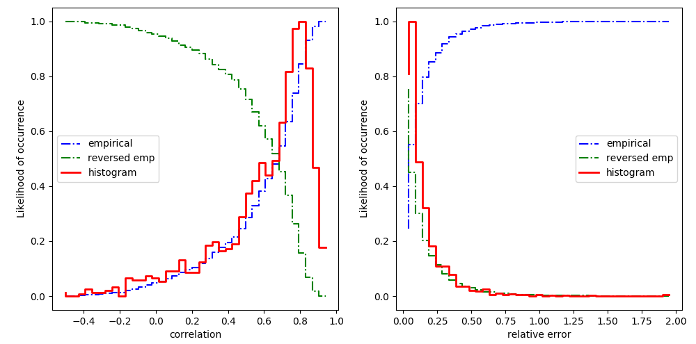kpi histograms

We indeed see that we have good performances on a freestander with drive but the satellite significantly drops overall performances

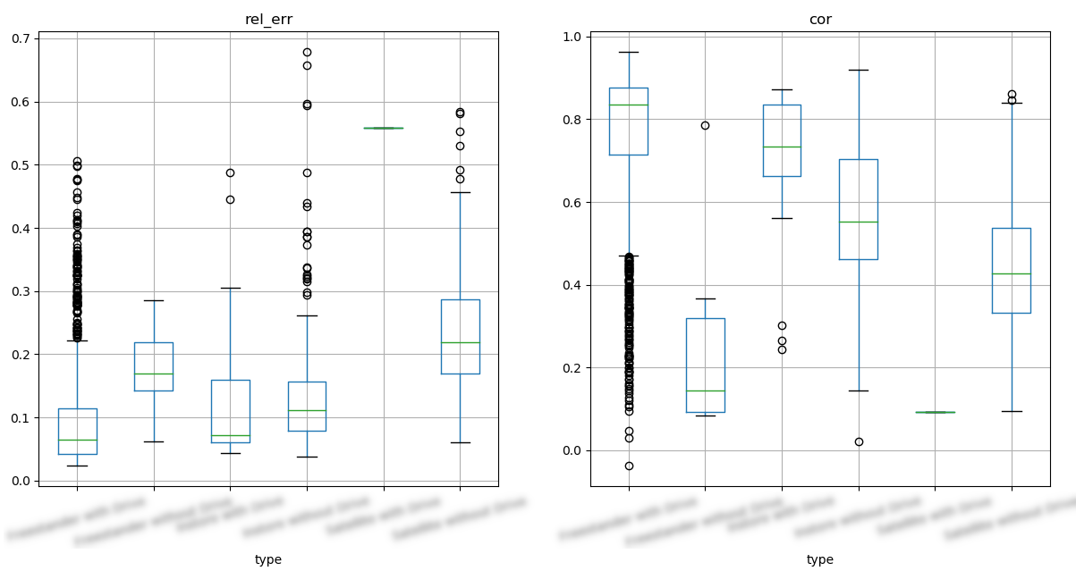kpi distribution per type